Download
1 / 65
680 likes | 752 Views
Explore the sources and drivers of economic growth, from the Solow Model to Endogenous Growth Theory. Understand the impact of government policies on long-term living standards, productivity growth, and capital input growth. Discover how historical data and growth accounting can shed light on the productivity slowdown and recent surge in U.S. productivity. Investigate the role of factors like ICT growth, government regulations, and technology adaptation in shaping economic growth. Dive into past technological revolutions and learn how adaptability drives long-term growth.

E N D
Chapter Outline • The Sources of Economic Growth • Long-Run Growth: The Solow Model • Endogenous Growth Theory • Government Policies to Raise Long-Run Living Standards
Long-Run Economic Growth • Introduction • Countries have grown at very different rates over long spans of time (Table 6.1) • We would like to explain why this happens
Table 6.1 Economic Growth in Eight Major Countries, 1870–2008
The Sources of Economic Growth • Production function Y = AF(K, N) (6.1) • Decompose into growth rate form: the growth accounting equation DY/Y = DA/A + aKDK/K + aNDN/N (6.2) • The a terms are the elasticities of output with respect to the inputs (capital and labor)
The Sources of Economic Growth • Interpretation • A rise of 10% in A raises output by 10% • A rise of 10% in K raises output by aK times 10% • A rise of 10% in N raises output by aN times 10% • Both aK and aN are less than 1 due to diminishing marginal productivity
The Sources of Economic Growth • Growth accounting • Four steps in breaking output growth into its causes (productivity growth, capital input growth, labor input growth) • Get data on DY/Y, DK/K, and DN/N, adjusting for quality changes • Estimate aK and aN from historical data • Calculate the contributions of K and N as aKDK/K and aNDN/N, respectively • Calculate productivity growth as the residual: DA/A=DY/Y – aKDK/K – aNDN/N
Table 6.2 The Steps of Growth Accounting: A Numerical Example
The Sources of Economic Growth • Growth accounting and the productivity slowdown • Denison’s results for 1929–1982 (text Table 6.3) • Entire period output growth 2.92%; due to labor 1.34%; due to capital 0.56%; due to productivity 1.02% • Pre-1948 capital growth was much slower than post-1948 • Post-1973 labor growth slightly slower than pre-1973
Table 6.3Sources of Economic Growth in the United States (Denison) (Percent per Year)
The Sources of Economic Growth • Productivity growth is major difference • Entire period: 1.02% • 1929–1948: 1.01% • 1948–1973: 1.53% • 1973–1982: –0.27% • Productivity growth slowdown occurred in all major developed countries
The Sources of Economic Growth • Application: the post-1973 slowdown in productivity growth • What caused the decline in productivity? • Measurement—inadequate accounting for quality improvements • The legal and human environment—regulations for pollution control and worker safety, crime, and declines in educational quality • Oil prices—huge increase in oil prices reduced productivity of capital and labor, especially in basic industries • New industrial revolution—learning process for information technology from 1973 to 1990 meant slower growth
The Sources of Economic Growth • Application: the recent surge in U.S. productivity growth • Labor productivity growth increased sharply in the second half of the 1990s • Labor productivity and TFP grew steadily from 1982 to 2008 (Fig. 6.1)
Figure 6.1 Productivity Levels, 1948-2011 Sources: Labor productivity: Bureau of Labor Statistics, Nonfarm Business Sector: Output Per Hour of All Persons, available at research.stlouisfed.org/fred2/series/OPHNFB. Total factor productivity: Bureau of Labor Statistics, Multifactor Productivity Trends, Table XG, available at ftp://ftp.bls.gov/pub/special.requests/opt/mp/prod3. mfptablehis.zip
Productivity • Labor productivity growth has generally exceeded TFP growth since 1995 (Fig. 6.2)
Figure 6.2 Productivity Growth, 1949-2011 Sources: Labor productivity: Bureau of Labor Statistics, Nonfarm Business Sector: Output Per Hour of All Persons, available at research. stlouisfed.org/fred2/series/ OPHNFB. Total factor productivity: Bureau of Labor Statistics, Multifactor Productivity Trends, Table XG, available at ftp://ftp.bls.gov/pub/special.requests/opt/mp/prod3.mfptablehis.zip
How can we relate this graph to our model? Use equations to relate the differing productivity concepts: Productivity
Productivity • So, labor productivity growth exceeds TFP growth because of faster growth of capital relative to growth of labor • ICT growth (information and communications technology) may have been a prime reason
Productivity • Why did ICT growth contribute to U.S. productivity growth, but not in other countries? • Government regulations • Lack of competitive pressure • Available labor force • Ability to adapt quickly
Productivity • Why was there such a lag between investment in ICT and growth in productivity? • Intangible capital • R&D • Firm reorganization • Worker training
Productivity • Similar growth in productivity experienced in past • Steam power, railroads, telegraph in late 1800s • Electrification of factories after WWI • Transistor after WWII • What matters most is ability of economy to adapt to new technologies
Long-Run Growth: The Solow Model • Two basic questions about growth • What’s the relationship between the long-run standard of living and the saving rate, population growth rate, and rate of technical progress? • How does economic growth change over time? Will it speed up, slow down, or stabilize?
The Solow Model • Setup of the Solow model • Basic assumptions and variables • Population and work force grow at same rate n • Economy is closed and G= 0 Ct=Yt – It (6.4) • Rewrite everything in per-worker terms: yt=Yt/Nt; ct=Ct/Nt; kt=Kt/Nt • kt is also called the capital-labor ratio
The Solow Model • The per-worker production function yt=f(kt) (6.5) • Assume no productivity growth for now (add it later) • Plot of per-worker production function (Fig. 6.3) • Same shape as aggregate production function
The Solow Model • Steady states • Steady state: yt, ct, and kt are constant over time • Gross investment must • Replace worn out capital, dKt • Expand so the capital stock grows as the economy grows, nKt It= (n+d)Kt (6.6)
The Solow Model • From Eq. (6.4), Ct=Yt – It=Yt – (n+d)Kt (6.7) • In per-worker terms, in steady state c=f(k) - (n+d)k (6.8) • Plot of c, f(k), and (n+d)k (Fig. 6.4)
Figure 6.4The relationship of consumption per worker to the capital–labor ratio in the steady state
The Solow Model • Increasing k will increase c up to a point • This is kG in the figure, the Golden Rule capital-labor ratio • For k beyond this point, c will decline • But we assume henceforth that k is less than kG, so c always rises as k rises
The Solow Model • Reaching the steady state • Suppose saving is proportional to current income: St=sYt, (6.9) where s is the saving rate, which is between 0 and 1 • Equating saving to investment gives sYt= (n+d)Kt (6.10)
The Solow Model • Putting this in per-worker terms gives sf(k) = (n+d)k (6.11) • Plot of sf(k) and (n+d)k (Fig. 6.5)
Figure 6.5 Determining the capital–labor ratio in the steady state
The Solow Model • The only possible steady-state capital-labor ratio is k* • Output at that point is y* = f(k*); consumption is c* = f(k*) – (n + d)k* • If k begins at some level other than k*, it will move toward k* • For k below k*, saving > the amount of investment needed to keep k constant, so k rises • For k above k*, saving < the amount of investment needed to keep k constant, so k falls
The Solow Model • To summarize: With no productivity growth, the economy reaches a steady state, with constant capital-labor ratio, output per worker, and consumption per worker
The Solow Model • The fundamental determinants of long-run living standards • The saving rate • Population growth • Productivity growth
The Solow Model • The fundamental determinants of long-run living standards • The saving rate • Higher saving rate means higher capital-labor ratio, higher output per worker, and higher consumption per worker (Fig. 6.6)
Figure 6.6The effect of an increased saving rate on the steady-state capital–labor ratio
The Solow Model • The fundamental determinants of long-run living standards • The saving rate • Should a policy goal be to raise the saving rate? • Not necessarily, since the cost is lower consumption in the short run • There is a trade-off between present and future consumption
The Solow Model • The fundamental determinants of long-run living standards • Population growth • Higher population growth means a lower capital-labor ratio, lower output per worker, and lower consumption per worker (Fig. 6.7)
Figure 6.7The effect of a higher population growth rate on the steady-state capital–labor ratio
The Solow Model • The fundamental determinants of long-run living standards • Population growth • Should a policy goal be to reduce population growth? • Doing so will raise consumption per worker • But it will reduce total output and consumption, affecting a nation’s ability to defend itself or influence world events
The Solow Model • The fundamental determinants of long-run living standards • Population growth • The Solow model also assumes that the proportion of the population of working age is fixed • But when population growth changes dramatically this may not be true • Changes in cohort sizes may cause problems for social security systems and areas like health care
The Solow Model • The fundamental determinants of long-run living standards • Productivity growth • The key factor in economic growth is productivity improvement • Productivity improvement raises output per worker for a given level of the capital-labor ratio (Fig. 6.8)
The Solow Model • The fundamental determinants of long-run living standards • Productivity growth • In equilibrium, productivity improvement increases the capital-labor ratio, output per worker, and consumption per worker • Productivity improvement directly improves the amount that can be produced at any capital-labor ratio • The increase in output per worker increases the supply of saving, causing the long-run capital-labor ratio to rise (Fig. 6.9)
Figure 6.9The effect of a productivity improvement on the steady-state capital–labor ratio
The Solow Model • The fundamental determinants of long-run living standards • Productivity growth • Can consumption per worker grow indefinitely? • The saving rate can’t rise forever (it peaks at 100%) and the population growth rate can’t fall forever • But productivity and innovation can always occur, so living standards can rise continuously • Summary: The rate of productivity improvement is the dominant factor determining how quickly living standards rise
Application: The growth of China • China is an economic juggernaut • Population 1.4 billion people • Real GDP per capita is low but growing (Table 6.4) • Starting with low level of GDP, but growing rapidly (Fig. 6.10)
Table 6.4 Economic Growth in China, Japan, and the United States