Download
1 / 23
270 likes | 671 Views
Conditional Convergence and Long-Run Economic Growth. Mr. Vaughan Income and Employment Theory (402). Conditional Convergence in Practice. Story thus far : Growth rate of capital per worker given by: ∆ k/k= ϕ[ k(0) , k*] (−) (+) Recall: y = A·f ( k )

E N D
Conditional Convergence and Long-Run Economic Growth Mr. Vaughan Income and Employment Theory (402)
Conditional Convergencein Practice Story thus far: • Growth rate of capital per worker given by: ∆k/k= ϕ[ k(0) , k*] (−) (+) • Recall: y = A·f( k) • So growth rate of real GDP per worker (capita) depends on initial/steady-state real GDP per worker (capita): ∆y/y = ϕ[ y(0), y*] (−) (+)
Solow Growth Model Evidence on Convergence • Problem • Hypothesis: Relationship between initial GDP per capita and subsequent growth rate should be negative. • Evidence: Not much pattern in data, and what exists appears positive. • PotentialExplanations: • Crummy Theoretical Model • Crummy Empirical Model
Conditional Convergencein Practice • Note: Conditional convergence clear when “other things equal.” • Variables influencing y* held constant: • Savings rate • Fertility rate • Measures of rule of law/democracy • Size of government • International openness (more exports/imports) • Changes in terms of trade • Investment in education and health • Average rate of inflation Horizontal axis shows real GDP per capita in 2000 dollars; vertical axis shows growth rate of real GDP per capita 1965-75 (matched with 1965 level), 1975-85 (matched with 1975 level), and 1985-95 (matched with 1985 level. Note: some countries appear three times.
Conditional Convergencein Practice Evidence suggests important to higher real growth rate: • Higher savings rate • Lower fertility rate • Better maintenance of rule of law • Smaller government consumption purchases • Greater international openness (i.e., more trade) • Improvement in terms of trade • Greater quality/quantity of education • Better health • Lower inflation “Democracy Effect” less clear: • Totalitarian starting point => Democratization raises growth. • After country reaches mid-range of democracy (i.e., Indonesia, Turkey, etc.), further democratization reduces growth.
Copenhagen Consensus 2008 Eight leading economists (5 Nobel Laureates) were asked: What policies would most advance global welfare – particularly in developing world – if $75 billion could be spent over four years? POLICY CATEGORY • Micronutrient supplements for children (vitamin A & zinc) Health & Nutrition • Doha development agenda Free Trade • Micronutrient fortification (iron & salt iodization) Health & Nutrition • Expanded immunization coverage for children Health & Nutrition • Bio-fortification Health & Nutrition • De-worming and other school-based nutrition programs Health & Nutrition / Education • Lowering the price of schooling Education • Increase / Improve girls’ schooling Education • Community-based nutrition promotions Health & Nutrition • Support for women’s reproductive role Health & Nutrition / Education Note: All 10 pro-growth policies!
Solow Growth ModelRecall SGM can explain: • Cross-country differences in steady-state living standards (real GDP per capita) • Cross-country differences in capital per worker. • Cross-country differences in growth rates (for similar countries) • Poor countries have higher growth rates of capital per worker and real GDP per capita because of convergence (lower k(0) than rich countries but same k*) • Cross-country differences in growth rates (for dissimilar countries) • Lack of convergence because k*’s differ. We have yet to explain why OECD countries can grow ≈ 2% per year for 100+years (because SGM says long-run growth rate of real GDP per capita = 0%).
Explaining Long-Run Economic GrowthRelaxing Assumption of Declining APK • Recall: in SGM, growth rate of capital per worker is: ∆k/k = s·(y/k) - (s·δ+ n) (3.16) …where declining APK (y/k) forces ∆k/k to zero in the long run. • Now, let’s relax assumption of declining APK (y/k). • Specifically, define capital to include human and infrastructure capital, and assume capital so defined is only factor of production. • So, standard production function: y = A·f(k) • Becomes: y = A·k(5.2 – “AK” Model) • Which (since 5.2 can be rewritten as A = y/k) implies: ∆k/k = s·A- (s·δ+ n) (5.4)
Explaining Long-Run Economic GrowthRelaxing Assumption of Declining APK • Note: • s(y/k) is not downward-sloping; it is constant = s·A. • s·Amore likely to exceed sδ+n if: • “s” higher • “A” higher • “δ” lower • “n” lower • Safe assumption (how many countries have long-term negative growth rates)? • Now: • Long-run growth rate of capital per worker (∆k/k) exceeds zero and equals: • s·A − (s·δ + n) • Growth rates of capital and real GDP per worker (∆k/k, ∆y/y) do not change as capital and real GDP per worker (“k” , “y”) rise. • Poor economies with low k(0) and y(0) may not grow faster than rich economies (i.e., no convergence). • Model Shortcomings • We do observe cross-convergence in cross-country data. • Most economists believe MPK and APK start falling at some point. • Let’s try introducing technical progress!
Explaining Long-Run Economic GrowthIntroducing Technological Progress • Cannot explain long-run growth in “k” and “y” with single increase in “A” – continuous increases needed. • Regular process of improvement in technology called technological progress. • In SGM, technological progress assumed to be continuous and exogenous (i.e., not explained bymodel) ∆A/A = g In words: Technology advances at some constant rate, “g.” (Later we will “endogenize” technological progress)
Explaining Long-Run Economic GrowthIntroducing Technological Progress Let’s do some algebra to make growth a function of continuous, exogenous technological progress: • Recall: ∆Y/Y = ∆A/A + α·(∆K/K) + (1-α)·(∆L/L) (3.3) • Substituting ∆A/A = g and ∆L/L = n in (3.3) yields: ∆Y/Y = g + α·(∆K/K) + (1-α)·n (5.5) • Recall: ∆y/y = ∆Y/Y - ∆L/L = ∆Y/Y - n(5.6)
Explaining Long-Run Economic GrowthIntroducing Technological Progress • Rewriting (5.6) as ∆Y/Y=∆y/y + nand substituting for ∆Y/Y in equation (5.5) yields: ∆y/y = g + α·(∆K/K) + [(1 - α)·n] - n • Which (with some manipulation) reduces to: ∆y/y = g + α·(∆K/K - n) (*) • Now, recall: ∆k/k = ∆K/K - ∆L/L (3.7) • So: ∆k/k = ∆K/K − n (5.7) • Substituting (5.7) in (*) yields: ∆y/y = g + α·(∆k/k) (5.8) In words: Real output per capita grows because of technological progress and growth in capital per worker.
Explaining Long-Run Economic GrowthIntroducing Technological Progress • Recall version of SGM with technology: ∆k/k = {s·[A·f(k)]/k} - (s·δ + n) (4.3) • Substituting (4.3) into (5.8) yields: ∆y/y = g + α·{[s·A·f(k)]/k} - (sδ + n)}(5.9) Key Equation: Growth rate of real GDP per worker with technical progress. NOTE: • In prior analysis, “A” was fixed, so increasing “k” reduced APK (y/k = A·f(k)/k) until ∆k/k = 0 (and ∆y/y = 0). Put another way, when g = 0 in (5.9), prior analysis holds – economy tends to steady state where ∆k/k = ∆y/y = 0. • Now, however, each increase in “A” (from g > 0) raises APK, in part, offsetting impact of rising “k” on APK (i.e., diminishing physical return to capital) – so economy does not necessarily tend to steady state where ∆k/k = ∆y/y = 0. • In equilibrium, forces balance (i.e., “k” increases in long run at constant rate and y/k doesn’t change). The resulting long-run growth rate of capital per worker and real GDP per capita is called steady-state growth.
Explaining Long-Run Economic GrowthIntroducing Technological Progress What drives steady-state growth in real GDP per capita? To answer, we will use algebra to derive equation for (∆y/y)* as function of exogenous variables. • In steady-state growth, y/k does not change – implying: (∆y/y)* = (∆k/k)* (5.10) • Recall: ∆y/y = g + α·(∆k/k) (5.8) • So: (∆y/y)* = g + α·(∆k/k)* (5.9) • Inserting equation (5.10) for (∆k/k)* in (5.9) yields: (∆y/y)* = g+ α·(∆y/y)* • Solving for (∆y/y)*yields: (∆y/y)* = g / (1 − α) (5.12) Key Equation: Steady-state growth rate for real GDP per capita, with technological progress.
Explaining Long-Run Economic GrowthIntroducing Technological Progress Steady-state growth rate with technological progress: (∆y/y)* = g / (1 − α) (5.12) Note: • Since 0 < α < 1, steady-state growth rate of real GDP per capita, (∆y/y)∗, exceeds rate of technological progress, “g”. For example, if α = ½ (capital’s share of national income = 50%), real output per capita grows at twice rate of technological progress. • Logic: In steady state (∆k/k)*> 0. Recall (5.9): ∆y/y* = g + α·(∆k/k)* ,i.e., per capita GDP grows by α·(∆k/k)* above “g”. • Recall (5.10): (∆y/y)* = (∆k/k)*. This implies: (∆k/k)* = g / (1 − α)(5.13) Key “take-away” from (5.12) and (5.13): Exogenous technological progress at rate ∆A/A= g produces long-term growth in capital per worker and real GDP per capita at rate “g / (1 − α)”. Technological progress offsets diminishing marginal/average productivity of capital, thereby allowing long-term positive growth of “k” and “y”.
Explaining Long-Run Economic GrowthIntroducing Technological Progress • NOTE: • In earlier analysis, k* was a constant asymptotically approached over time. • Now, k* grows over time by: • (∆k/k)* = g/(1−α) • Model still has transition in which k(0) asymptotically approaches k* over time. • “Catching” (∆k/k)* requires (∆k/k)> g/(1−α)
Explaining Long-Run Economic GrowthIntroducing Technological Progress • NOTE: • Convergence now depends on whether countries have same growth rate of steady-state capital per worker, (∆k/k)*,rather than same level of k*. • In figure, poor country represented by red line, rich country by green line. Both countries have same steady-state growth rate for capital per worker, k*. • Growth in capital per worker from initial state is higher for poor country k1(0)than for rich country k2(0). • Put another way, convergence holds.
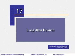
Explaining Long-Run Economic GrowthIntroducing Technological Progress • NOTE: • In figure, poor country represented by red line, rich country by green line. Now countries have different steady-state growth rates of capital per worker (blue dashed line for rich country, k2*, and red dashed line for poor country, k1*) • Now, growth rates of capital per worker (and real GDP per capita) in poor country need not be higher than growth rates in rich country. • Put another way, convergence need not hold any longer. • Implication: • SGM (with or without continuous exogenous technological progress) can explain failure of poor countries to converge on rich countries.
Solow Growth ModelThe Scorecard • Data Patterns to Explain: • Significant differences in steady-state living standards (real GDP per capita) across countries: • Cross-country differences in capital per worker. • Cross-country differences in growth rates (for similar countries) • Poor countries have higher growth rates of capital per worker and real GDP per capita because of convergence [lower k(0) than rich countries but same k* or growth rate of k*] • Cross-country differences in growth rates (for dissimilar countries) • Lack of convergence because level of k* or growth rates of k* differ. • Ability of OECD countries to maintain long-term growth rates of real GDP per capita ≈ 2% for 100+ years. • Continuous technological progress. • Only loose end: Technological progress is exogenous!
Endogenous Growth Theory(founded by Paul Romer) • Called “endogenous” because models: • Extend SGM to explain rate of technological progress, and… • Technological progress produces positive long-run growth of capital per worker/real GDP per capita [as in SGM]. • Most endogenous growth models driven by investments in research and development (R&D): • Technological progress represented by increases in “A” (in SGM framework). • MoreR&D implies more technological progress (discovery of new/better products or superior methods of production), other things equal. • Marginal returns on R&D-driven technological progress do not decline (i.e., good ideas unlimited) => produces constant growth rate (g) for “A” (like SGM). • Other things equal, factors raising private-sector return to R&D lead to more R&D: • Lower costs of R&D (e.g., government subsidies of research) • Higher potential sales revenues/lower production costs from R&D investment (e.g., larger market for selling fruits of R&D => explain links between free trade and growth). • More secure (and long-lasting) intellectual property rights over use of inventions from R&D.
Endogenous Growth Theory(founded by Paul Romer) Empirical Evidence: • Countries spending most on R&D, other things equal, have higher growth rates of real GDP per capita. • Advanced countries spend most on R&D (explains high long-term OECD growth rates). • Poor countries can raise level of technology by imitating/adapting innovations from other countries (Diffusion of Technology) • Another potential source of convergence (high growth rate initially, but opportunities for additional profitable imitation decline). • Rate of technological innovation to developing country is high, other things equal, when that country : • Trades extensively with rich countries. • Has high education levels. • Has well-functioning legal/political systems. Helps explain high growth rates of East Asian countries since 1960!
Thought Questions • Based on what you have learned, what explains poor growth record in Sub-Saharan Africa? • What policies would you recommend to boost growth/alleviate poverty and why? *** • What policies would you recommend to President Obama to boost long-term U.S. growth?
Questionsover Conditional Convergence and Long-Run Economic Growth Mr. Vaughan Income and Employment Theory (402)