Download
1 / 27
270 likes | 295 Views
By M. J. Kavaya, G. J. Koch, F. Amzajerdian, B. W. Barnes, R. E. Davis, U. N. Singh NASA Langley Research Center R. G. Frehlich Univ. of Colorado to Working Group on Space-Based Lidar Winds 28 June – 1 July, 2005 Welches, Oregon.

E N D
By M. J. Kavaya, G. J. Koch, F. Amzajerdian, B. W. Barnes, R. E. Davis, U. N. Singh NASA Langley Research Center R. G. Frehlich Univ. of Colorado to Working Group on Space-Based Lidar Winds 28 June – 1 July, 2005 Welches, Oregon Estimating Space Performance of a Coherent Doppler Wind Lidar by Inverting Ground Performance
One component of properly designing and persuasively selling an orbiting Doppler wind lidar mission is to be able to predict performance We need to be confident of our performance predicting simulations One valuable approach is bottoms-up simulations from first principles; this approach was advanced by the GTWS effort This paper discusses an independent way to validate the bottoms up simulation of coherent Doppler wind lidar by using the information from an actual ground-based Doppler lidar system and the wind data that it gathers We appreciate the IPO support that enabled the ground based data used here Motivation
Begin with actual data taken vertically Look at the performance at 2 km Ratio the ground and space equations to cancel terms that are common Compare the predicted signal from the space geometry (833 km, 30 deg) to what is required for operation What We Want To Do
Include every physical process that affects the wind velocity measurement performance Don’t include any physical process more than once Harder Than It Seems
LaRC Ground Wind Measurement • zenith viewing • 20 pulses averaged • 5 Hz pulse repetition freq (PRF) • 91 mJ pulse energy • 50k samples at 500 Ms/s • Note each wind measurement uses 1.8 J of optical energy, 4 seconds of time, and a 15-cm-diameter collection mirror. Winds are consistently measured to 7-8 km altitude, and occasionally to 9-10 km. The 20 minutes shown here consist of 300 vertical wind vertical profiles. • Winds strong and variable with clear skies. • On wind plot red is updraft, blue is downdraft. • Gray color is outside the wind speed range on the y axis. • Signal power is not corrected for range squared
Coherent Doppler Wind Lidar SNR Equation F1 = eff. no. coherent photoelectrons per shot per range gate Dp LSE = Lidar System Efficiency, ATM = Atmosphere, SB = Search Bandwidth SBF = Search Bandwidth, Frequency Units; [BSBV = BSBF * (l/2)]; OBS = Observation See, e.g., Frehlich and Kavaya, Appl. Opt. 30, 5325 (1991). Eqs. (92, 117, 119) Frehlich, J. Atmos. Oceanic Technol. 21, 905 (2004)
All The Gory Details - 1 Light Intensity Transmission (T): 0.51 Light Intensity Transmission (T) Coefficients, Transmit Path: 0.776 = 0.955 0.99 0.99 0.95 0.9 1 0.97 1 Light Intensity Transmission (T) Coefficients, Receive Path: 0.658 = 1 0.9 0.95 0.99 0.9 0.89 0.97 1 Space design numbers
All The Gory Details - 2 Aberration (A) Loss: 0.840 Aberration (A) Loss Factors, Transmit Path: 0.917 = Ö0.95 Ö0.95 Ö0.95 Ö1 Ö0.98 Aberration (A) Loss Factors, Receive Path: 0.917 = Ö1 Ö0.95 Ö0.95 Ö0.95 Ö0.98
All The Gory Details - 3 Heterodyne Detection (H) Loss Factors: 0.294 = 0.95 1 0.42 0.98 0.8 0.97 0.97 1 Estimated Space LSE = 12.6% Transmitter/Receiver Misalignment (M) Loss Factors: 0.5 = 0.707 0.707
Converting Ground Performance to Space Prediction Ground-Based Equation: Green = Ground Space-Based Equation: Orange = Orbit
Converting Ground Performance to Space Prediction We need to form a ratio so that common terms will cancel Space to Ground SNR Ratio: Use an actual ground measurement at z = 2 km, consider space measurement at z = 2 km, assume same wavelength & aerosol backscatter. Adjust for different parameter values between the ground lidar and the notional space lidar
Converting Ground Performance to Space Prediction Space to Ground SNR Ratio: Now start calculating individual ratios: Dz = 1 km, 34 deg: Dp = 1212 m
Converting Ground Performance to Space Prediction Use 1 if optic not used Light Intensity Transmission (T): = 1 = 1 = 1 = 1 = 1 = 1 = 1 = 1 = 1 = 1 Not counting likely lower values in ground system than space for cancelled terms
Converting Ground Performance to Space Prediction Aberration (A) Loss: = 1 = 1 = 1 = 1 = 1 = 1 Not counting likely lower values in ground lidar than space lidar for cancelled terms AT,FOC*AR,FOC = 0.179 when D = 15 cm, F = ¥, R = 2 km
Converting Ground Performance to Space Prediction Heterodyne Detection (H) Loss Factors: = 1 Not counting likely lower values in ground lidar than space lidar for cancelled terms Assume ground loss from refractive turbulence (RT) ~ 3 dB Transmitter/Receiver Misalignment (M) Loss Factors: Ground system misalignment not known, assume none = 1 = 1
Converting Ground Performance to Space Prediction Now gather all the ratios and multiply them: An average value of F1,G was 1000, therefore F1,O > 0.73 • The required value of F1,O is 0.8 • assuming: • 50% good estimates (or 1.9 for 90% good) • 2 m/s eff. spectral width • 120 shots accumulated • 20 m/s LOS search space (35 m/s horiz. search space) J
Converting Ground Performance to Space Prediction • Possible further adjustments in performance prediction: • Signal processing in space will work better than what we now do • The horizontal search space can probably be smaller • The ground turning mirror is causing a 3 dB loss, which shouldn’t happen is space • The ground polarization losses are probably worse than space • The ground transmission losses are probably worse than space • The ground aberration losses are probably worse than space • There may have been unknown ground misalignment losses • All the above would improve space performance
Converting Ground Performance to Space Prediction Conclusions • The inversion of ground-based data to predict space-based performance (833 km, 30 deg, 20 cm, 120 shots, 2 km height, 50% good estimates) closely matches the performance prediction from Emmitt
Back Up Slides 1/7/2020 1/7/2020 19 LaRC/Kavaya-
Converting Ground Performance to Space Prediction SNRSB Values
Transmit Path Intensity Transmission • 0.955 Basic aperture • 0.99 T/R switch – pol. BS incl. polarization misal. • 0.99 T/R switch - quarter wave plate • 0.95 Telescope • 0.9 Scanner • 1 Pressure window (no PW) • 0.97 All other optics • 1 All obscurations (none) • __________________________________ • 0.776 Sub product New since ISAL/IMDC 1/7/2020 23 LaRC/Kavaya-
Receiver Path Intensity Transmission • 1 Pressure window (no PW) • 0.9 Scanner • 0.95 Telescope • 0.99 T/R switch - quarter wave plate • 0.9 T /R switch – pol. BS incl. pol. misal. • 0.89 LO/signal beam splitter (BS) • 0.97 All other optics • 1 All obscurations (none) • 1 Fibers, ports, & coupler (no fibers) • _________________________________ • 0.658 Sub product • __________________________________ • 0.511 T & R transmission sub product 1/7/2020 24 LaRC/Kavaya-
SNR Reducing Aberration Factors • 0.95 Telescope, 2 passes • 0.95 Telescope, incorrect focus setting • 0.95 Scanner, 2 passes • 1 Pressure window, 2 passes (no PW) • 0.98 Other optics, some 1 pass, some 2 pass • ______________________________________ • 0.840 Aberration sub product 1/7/2020 25 LaRC/Kavaya-
SNR Reducing Detection Terms • 0.95 Laser beam spatial quality • 1 Detector truncation • 0.42 Mixing efficiency • 0.98 XMTR/RECR polarization mismatch • 0.8 Detector quantum efficiency at IF frequency • 0.97 Detector nonlinearity factor • 0.97 Nondominating shot noise factor • 1 Refractive turbulence factor • ___________________________________ • 0.294 Detection sub product 1/7/2020 26 LaRC/Kavaya-
0.511 T/R intensity transmission factor • 0.840 Aberration sub product • 0.294 Detection sub product • 0.126 Lidar System Efficiency (LSE) • 0.5 Transmitter/receiver angle misalignment factor (2.053 mrad total 1s misalignment angle outside lidar, 4 ms) • (Assign half to lidar, half to spacecraft, 1.45 mrad each) • 0.707 Lidar portion of T/R angle misalignment ML • 0.707 Spacecraft portion of T/R angle misalignment factor, MSC 1/7/2020 27 LaRC/Kavaya-