Download
1 / 14
140 likes | 165 Views
Investigating chaotic phenomena at the edge of LHD magnetic fields using specialized coordinate grids and surface interpolation techniques. Examination of stable and unstable periodic curves, irrational flux effects, and diagnostic criteria for magnetic field stability.

E N D
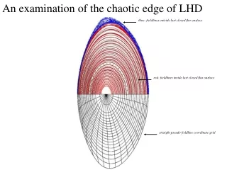
An examination of the chaotic edge of LHD blue: fieldlines outside last closed flux surface red: fieldlines inside last closed flux surface straight pseudo fieldline coordinate grid
An examination of the chaotic edge of LHD (10,6) island chain , and (10,6) ghost-surface near critical cantori last closed flux surface (10,7) island chain , and (10,7) ghost-surface
The magnetic field is given in cylindrical coordinates, and arbitrary, toroidal coordinates are introduced. ϑ ζ ρ Begin with circular cross section coordinates, centered on the magnetic axis. In practice, we will have a discrete set of toroidal surfaces that will be used as “coordinate surfaces”. The Fourier harmonics, Rm,n & Zm,n, of a discrete set of toroidal surfaces are interpolated using piecewise cubic polynomials. A regularization factor is introduced, e.g. to ensure that the interpolated surfaces do not overlap near the coordinate origin=magnetic axis. If the surfaces are smooth and well separated, this “simple-minded” interpolation works.
A magnetic vector potential, in a suitable gauge, is quickly determined by radial integration. hereafter, we will use the commonly used notation ψ is the toroidal flux, and χ is called the magnetic field-line Hamiltonian
The magnetic field-line action is the line integral of the vector potential piecewise-constant, piecewise-linear the piecewise-linear approximation allows the cosine integral to be evaluated analytically, i.e. method is FAST To find extremizing curves, use Newton method to set ∂ρS=0, ∂ϑS=0 reduces to , which can be solved locally, tridiagonal Hessian, inverted in O(N) operations, i.e. method is FAST Not required to follow magnetic field lines, and does not depend on coordinate transformation.
The trial-curve is constrained to be periodic, and a family of periodic curves is constructed. Usually, there are only the “stable” periodic field-line and the “unstable” periodic field line, ϑO “stable” periodic orbit ϑX “unstable” periodic orbit ρ poloidal angle, ϑ However, we can “artificially” constrain the poloidal angle, i.e. ϑ(0)=given constant, and search for extremizing periodic curve of the constrained action-integral A rational, quadratic-flux minimizing surface is a family of periodic, extremal curves of the constrained action integral, and is closely to related to the rational ghost-surface, which is defined by an action-gradient flow between the minimax periodic orbit and the minimizing orbit.
The “upward” flux = “downward” flux across a toroidal surface passing through an island chain can be computed. the total flux across any closed surface of a divergence free field is zero. toroidal angle, ζ ρ poloidal angle, ϑ consider a sequence of rationals, p/q, that approach an irrational, If Ψp/q→∆, where ∆≠ 0, then the KAM surface is “broken”, and Ψp/q is the upward-flux across the cantorus
The diagnostics include: • Greene’s residue criterion: the existence of an irrational surface can be determined by calculating the stability of nearby periodic orbits. • Chirikov island overlap: flux surfaces are destroyed when magnetic islands overlap. • Cantori: can present effective, partial barriers to fieldline transport, and cantori can be approximated by high-order periodic orbits.
The construction of chaotic coordinates simplifies anisotropic diffusion free-streaming along field line particle “knocked” onto nearby field line In chaotic coordinates, the temperature becomes a surface function, T=T(s), where s labels invariant (flux) surfaces or almost-invariant surfaces. If T=T(s), the anisotropic diffusion equation can be solved analytically, where c is a constant, and is related to the quadratic-flux across an invariant or almost-invariant surface, is a geometric coefficient. An expression for the temperature gradient in chaotic fieldsS.R. Hudson, Physics of Plasmas, 16:010701, 2009 Temperature contours and ghost-surfaces for chaotic magnetic fieldsS.R.Hudson and J.BreslauPhysical Review Letters, 100:095001, 2008 When the upward-flux is sufficiently small, so that the parallel diffusion across an almost-invariant surface is comparable to the perpendicular diffusion, the plasma cannot distinguish between a perfect invariant surface and an almost invariant surface
List of publications, http://w3.pppl.gov/~shudson/ Generalized action-angle coordinates defined on island chainsR.L.Dewar, S.R.Hudson and A.M.GibsonPlasma Physics and Controlled Fusion, 55:014004, 2013 Unified theory of Ghost and Quadratic-Flux-Minimizing SurfacesRobert L.Dewar, Stuart R.Hudson and Ashley M.GibsonJournal of Plasma and Fusion Research SERIES, 9:487, 2010 Are ghost surfaces quadratic-flux-minimizing?S.R.Hudson and R.L.DewarPhysics Letters A, 373(48):4409, 2009 An expression for the temperature gradient in chaotic fieldsS.R.HudsonPhysics of Plasmas, 16:010701, 2009 Temperature contours and ghost-surfaces for chaotic magnetic fieldsS.R.Hudson and J.BreslauPhysical Review Letters, 100:095001, 2008 Calculation of cantori for Hamiltonian flowsS.R.HudsonPhysical Review E, 74:056203, 2006 Almost invariant manifolds for divergence free fieldsR.L.Dewar, S.R.Hudson and P.PricePhysics Letters A, 194(1-2):49, 1994
The fractal structure of chaos is related to the structure of numbers Farey Tree alternating path alternating path (excluded region)
For non-integrable fields, field line transport is restricted by KAM surfaces and cantori KAM surface delete middle third complete barrier cantor set partial barrier gap Calculation of cantori for Hamiltonian flows S.R. Hudson, Physical Review E 74:056203, 2006 • KAM surfaces are closed, toroidal surfaces that stop radial field line transport • Cantori have “holes” or “gaps”; but cantori can severely “slow down” radial field line transport • Example: all flux surfaces destroyed by chaos, but even after 100 000 transits around torus the field lines cannot get past cantori “noble” cantori (black dots) radial coordinate
Chaotic coordinates “straighten out” chaos Poincaré plot of chaotic field (in action-angle coordinates of unperturbed field) Poincaré plot of chaotic field in chaotic coordinates old radial coordinate → new radial coordinate → old angle coordinate → new angle coordinate → phase-space is partitioned into (1) regular (“irrational”) regions with “good flux surfaces”, temperature gradients and (2) irregular (“ rational”) regions with islands and chaos, flat profiles Generalized magnetic coordinates for toroidal magnetic fields S.R. Hudson, Doctoral Thesis, The Australian National University, 1996
Chaotic coordinates simplify anisotropic transport The temperature is constant on ghost surfaces, T=T(s) 1. Transport along the magnetic field is unrestricted → consider parallel random walk, with long steps collisional mean free path 2. Transport across the magnetic field is very small →consider perpendicular random walk with short steps Larmor radius 3. Anisotropic diffusion balance 4. Compare solution of numerical calculation to ghost-surfaces 5. The temperature adapts to KAM surfaces,cantori, and ghost-surfaces! i.e. T=T(s), where s=const. is a ghost-surface from T=T(s,,) to T=T(s) is a fantastic simplification, allows analytic solution free-streaming along field line particle “knocked” onto nearby field line 212 ×212 = 4096 ×4096 grid points (to resolve small structures) cold ghost-surface ghost-surface isotherm Temperature contours and ghost-surfaces for chaotic magnetic fields S.R. Hudson et al., Physical Review Letters, 100:095001, 2008 Invited talk 22nd IAEA Fusion Energy Conference, 2008 Invited talk 17th International Stellarator, Heliotron Workshop, 2009 An expression for the temperature gradient in chaotic fields S.R. Hudson, Physics of Plasmas, 16:100701, 2009 hot