3.2. Cournot Model
3.2. Cournot Model. Matilde Machado. 3.2. Cournot Model. Assumptions: All firms produce an homogenous product The market price is therefore the result of the total supply (same price for all firms) Firms decide simultaneously how much to produce

3.2. Cournot Model
E N D
Presentation Transcript
3.2. Cournot Model Matilde Machado
3.2. Cournot Model Assumptions: • All firms produce an homogenous product • The market price is therefore the result of the total supply (same price for all firms) • Firms decide simultaneously how much to produce • Quantity is the strategic variable. If OPEC was not a cartel, then oil extraction would be a good example of Cournot competition. Agricultural products? http://www.iser.osaka-u.ac.jp/library/dp/2010/DP0766.pdf ? • The equilibrium concept used is Nash Equilibrium (Cournot-Nash) 3.2. Cournot Model
3.2. Cournot Model Graphically: • Let’s assume the duopoly case (n=2) • MC=c • Residual demand of firm 1: RD1(p,q2)=D(p)-q2. The problem of the firm with residual demand RD is similar to the monopolist’s. 3.2. Cournot Model
3.2. Cournot Model Graphically (cont.): P p* D(p) MC RD1(q2) = Residual demand q*1= R1(q2) q2 MR 3.2. Cournot Model
3.2. Cournot Model Graphically (cont.): q*1(q2)=R1(q2) is the optimal quantity as a function of q2 Let’s take 2 extreme cases q2: Case I: q2=0 RD1(p,0)=D(p) whole demand q*1(0)=qM Firm 1 should produce the Monopolist’s quantity 3.2. Cournot Model
3.2. Cournot Model D(p) Case 2: q2=qcRD1(p,qc)=D(p)-qc c Residual Demand qc c D(p) MR<MCq*1=0 qc MR 3.2. Cournot Model
3.2. Cournot Model Note: If both demand and cost functions are linear, reaction function will be linear as well. q1 Reaction function of firm 1 qM q*1(q2) qc q2 3.2. Cournot Model
3.2. Cournot Model If firms are symmetric then the equilibrium is in the 45º line, the reaction curves are symmetric and q*1=q*2 q1 qc q1=q2 q*2(q1) qM q*1 E q*1(q2) 45º qM qc q*2 q2 3.2. Cournot Model
3.2. Cournot Model Comparison between Cournot, Monopoly and Perfect Competition qM<qN<qc q1 qc q*2(q1) q1+q2=qN q1+q2=qc qM q*1(q2) qM q1+q2=qN qc q2 q1+q2=qM 3.2. Cournot Model
3.2. Cournot Model Derivation of the Cournot Equilibrium for n=2 P=a-bQ=a-b(q1+q2) MC1=MC2=c For firm 1: Takes the strategy of firm 2 as given, i.e. takes q2 as a constant. Note the residual demand here Reaction function of firm 1: optimal quantity firm 1 should produce given q2. If q2 changes, q1 changes as well. 3.2. Cournot Model
3.2. Cournot Model We solve a similar problem for firm 2 and obtain a system of 2 equations and 2 variables. If firms are symmetric, then Solution of the Symmetric equilibrium 3.2. Cournot Model
3.2. Cournot Model Solution of the Symmetric equilibrium 3.2. Cournot Model
3.2. Cournot Model Comparing with Monopoly and Perfect Competition Where we obtain that: In perfect competition prices increase 1-to-1 with costs. 3.2. Cournot Model
3.2. Cournot Model In the Case of n2 firms: If all firms are symmetric: 3.2. Cournot Model
3.2. Cournot Model Total quantity and the equilibrium price are: If the number of firms in the oligopoly converges to ∞, the Nash-Cournot equilibrium converges to perfect competition. The model is, therefore, robust since with n→ ∞ the conditions of the model coincide with those of the perfect competition. 3.2. Cournot Model
3.2. Cournot Model DWL in the Cournot model = area where the willingness to pay is higher than MC pN DWL c QN qc When the number of firms converges to infinity, the DWL converges to zero, which is the same as in Perfect Competition. The DWL decreases faster than either price or quantity (rate of n2) 3.2. Cournot Model
3.2. Cournot Model In the Asymmetric duopoly case with constant marginal costs. The FOC (from where we derive the reaction functions): Replace q2 in the reaction function of firm 1 and solve for q1 3.2. Cournot Model
3.2. Cournot Model In the Asymmetric duopoly case with constant marginal costs. Which we replace back in q2: 3.2. Cournot Model
3.2. Cournot Model From the equilibrium quantities we may conclude that: If c1<c2 (i.e. firm 1 is more efficient): In Cournot, the firm with the largest market share is the most efficient 3.2. Cournot Model
3.2. Cournot Model From the previous result, the more efficient firm is also the one with a larger price-Mcost margin: 3.2. Cournot Model
3.2. Cournot Model Comparative Statics: The output of a firm ↓ when: ↑ own costs ↓ costs of rival q2 ↑c1 Shifts the reaction curve of firm 1 to the left R1 E’ E ↑q*2 and ↓q*1 R2 q1 3.2. Cournot Model
3.2. Cournot Model Profits are: Increase with rival’s costs Decrease with own costs Symmetric to firm 2. 3.2. Cournot Model
3.2. Cournot Model More generally… for any demand and cost function. There is a negative externality between Cournot firms. Firms do not internalize the effect that an increase in the quantity they produce has on the other firms. That is when ↑qi the firm lowers the price to every firm in the market (note that the good is homogenous). From the point of view of the industry (i.e. of max the total profit) there will be excessive production. Externality: firms only take into account the effect of the price change in their own output. Then their output is higher than what would be optimal from the industry’s point of view. 3.2. Cournot Model
3.2. Cournot Model If we define the Lerner index of the market as: Is the Herfindhal Concentration Index 3.2. Cournot Model
3.2. Cournot Model The positive relationship between profitability and the Herfindhal Concentration Index under Cournot: Remember the FOC for each firm in that industry can be written as: The Industry-wide profits are then: The concentration index is up to a constant an exact measure of industry profitability. 3.2. Cournot Model
3.2. Cournot Model Note: The Cournot model is often times criticized because in reality firms tend to choose prices not quantities. The answer to this criticism is that when the cournot model is modified to incorporate two periods, the first where firms choose capacity and the second where firms compete in prices. This two period model gives the same outcome as the simple Cournot model. 3.2. Cournot Model