Image analysis with EBImage
This presentation introduces EBImage, a set of quantitative image processing tools for R, enabling advanced image analysis. Key functionalities include image reading, writing, and rendering, alongside sophisticated processing techniques such as linear operators and morphological transformations. The main goal is to extract cellular descriptors and classify cells through automatic phenotyping. Using techniques like object detection, feature extraction, and segmentation, users can efficiently analyze multidimensional images, enhancing biological research capabilities.


Image analysis with EBImage
E N D
Presentation Transcript
Image analysis with EBImage Gregoire Pau, EMBL Heidelberg gregoire.pau@embl.de
Introduction • EBImage • Set of quantitative image processing tools • Image reading/writing/rendering • Image processing (linear operators, matrix algebra, morphology) • Object detection • Features extraction • Goal • Extract cellular descriptors • Classify cells • Automatic phenotyping • Process/transform images
Image representation • Image object • Array of intensity values • Lena: 512x512 matrix
Image representation • Multi-dimensionnal array • 2D: spatial dimensions • Other dimensions: replicate, time point, color, condition, z-slice Nuclei 4 replicates r0 r1 r2 r3 Lena 3 color channels R G B
Image rendering • Rendering dissociated from representation Sequence of images Color images Nuclei 4 replicates r0 r1 r2 Lena 3 color channels R G B
IO • Functions readImage(), writeImage() • Reads an image, returns an array • Supports 80 formats (JPEG, TIFF, PNG…) • Supports HTTP, sequences of images • Example: image format conversion • x = readImage('sample-001-02a.tif') • writeImage(x, 'sample-001-02a.jpeg', quality=95)
Display • Function display() • GTK+ interactive: zoom, scroll, animate • Supports RGB color channels and sequence of images
Matrix algebra • Let denote lena by x • Let us consider x • Adjust brightness, contrast and gamma-factor x x+0.5 3*x (x+0.2)3
Spatial transformation • Cropping, thresholding, rotation, resize x[45:56, 98:112] x > 0.5 resize(x, w=128) rotate(x, 30)
Thresholding • Global thresholding • Building block tool to segment cells x x > 0.3
Linear filter • 2D convolution with filter2() • Low-pass filter • Smooth images, remove artefacts x 1 1 1 1 1 1 1 1 1 x
Linear filter • High-pass filter • Detect cell edges x -1 -1 -1 -1 8 -1 -1 -1 -1 x
Nuclei segmentation • Global thesholding + labelling • Function bwlabel() • Labels connected sets (objects) from a binary image • Every pixels of an object is set to an unique integer value • max(bwlabel(x)) gives the number of detected objects x>0.2 bwlabel(x>0.2) x
Better segmentation • Adaptive thresholding + mathematical opening + holes filling • xb = thresh(x[,,1], 10, 10, 0.05) • kern = makeBrush(5, shape='disc') • xb = dilate(erode(xb, kern), kern) • xl = bwlabel(fillHull(nuct2)) xb xl x
Cell segmentation • Using Voronoi segmentation with propagate() • Image gradient-based metric
Cell segmentation • Combining channels and segmentation masks
Features extraction • Function getFeatures() • Extracts features from image objects • Geometric, image moment based features • Texture based features (Zernike moments, Haralick features) 100 features g.x g.y g.s g.p g.pdm g.pdsd g.effr g.acirc [1,] 123.1391 3.288660 194 67 9.241719 4.165079 7.858252 0.417525 [2,] 206.7460 9.442248 961 153 20.513190 7.755419 17.489877 0.291363 [3,] 502.9589 7.616438 219 60 8.286918 1.954156 8.349243 0.155251 [4,] 20.1919 22.358418 1568 157 22.219461 3.139197 22.340768 0.116709 [5,] 344.7959 45.501992 2259 233 35.158966 15.285795 26.815332 0.501106 [6,] 188.2611 50.451863 2711 249 28.732680 6.560911 29.375808 0.168941 [7,] 269.7996 46.404036 2131 180 26.419631 5.529232 26.044546 0.193805 [8,] 106.6127 58.364243 1348 143 21.662879 6.555683 20.714288 0.264836 [9,] 218.5582 77.299007 1913 215 25.724580 6.706719 24.676442 0.243073 [10,] 19.1766 81.840147 1908 209 26.303760 7.864686 24.644173 0.304507 [11,] 6.3558 62.017647 340 68 10.314127 2.397136 10.403142 0.188235 [12,] 58.9873 86.034128 2139 214 27.463158 6.525559 26.093387 0.207106 [13,] 245.1087 94.387405 1048 123 18.280901 2.894758 18.264412 0.112595 [14,] 411.2741 109.198678 2572 225 28.660816 7.914664 28.612812 0.224727 [15,] 167.8151 107.966014 1942 160 24.671533 2.534342 24.862779 0.084963 [16,] 281.7084 121.609892 2871 209 31.577270 6.470767 30.230245 0.128874 [17,] 479.2334 143.098241 1649 183 23.913630 6.116630 22.910543 0.248635 [18,] 186.5930 146.693122 2079 199 27.280908 6.757808 25.724818 0.195286 [19,] 356.7303 148.253418 3145 285 34.746206 11.297632 31.639921 0.313513 [20,] 449.2436 147.798319 119 37 5.873578 1.563250 6.154582 0.243697 ... 76 cells
siRNA screen • 3 immunostains: DNA, Actin, Tubulin siRluc siCLSPN
Features • Cell size • Median cell size of 1024 um2 (siRluc) and 1517 um2 (siCLSPN) • Wilcoxon rank sum test, P-value < 10-12