Enhancing Image Analysis through Signal-to-Symbol and Symbol-to-Symbol Transformations
340 likes | 460 Views
This document explores the methodologies for image analysis involving signal-to-symbol and symbol-to-symbol transformations, which are crucial for extracting meaningful information from images. It covers global information extraction, pixel value distributions, and connected components, leading into middle-level and high-level interpretation. Key techniques such as intensity histograms, thresholding, contrast stretching, and histogram equalization are discussed, illustrating their roles in image classification, including both supervised and unsupervised methods. Practical applications, such as remote sensing classification, demonstrate the methodologies' effectiveness.

Enhancing Image Analysis through Signal-to-Symbol and Symbol-to-Symbol Transformations
E N D
Presentation Transcript
Signal-to-symbol transformation/ feature extraction Symbol-to-symbol transformation/ feature extraction Image Analysis • Abstract • Extract usable global information from the image. • The image analysis operators extract useful information • Pixel value distribution • Classified pixels • Connected components • This is part of the middle level image interpretation and used for the high level image interpretation.
Count Intensity Intensity Histogram (I) • Brief Description • A graph showing the number of pixels in an image at each different intensity value • This shows the distribution of pixels graphically.
Thresholded Image Original Image Histogram Intensity Histogram (II) • How It Works • The image is scanned in a single pass and a running count of the number of pixels found at each intensity value is kept. • Guideline for Use • One of the common uses is to decide what value of threshold to use when converting a grayscale image to a binary one.
Intensity Histogram (III) • Example: Thresholding • There is a significant illumination gradient across the image (a), and it blurs out the histogram. • No longer possible to select a single global threshold that will neatly segment the object from its background. • Two failed thresholding segmentations are shown in (c) and (d). (c) Threshold 80 (a) Illuminated Image (b) Histogram (d) Threshold 120
(a) Original Image (b) Result of Contrast Stretching Intensity Histogram (IV) • Example: Contrast Stretching • Contrast stretching takes an image in which the intensity values do not span the full intensity range and stretches its values linearly. • Histogram of (a) shows that most of the pixels have rather high intensity values. • Contrast stretching the image yields (b) which has a clearly improved contrast .
(A) Original Image (B) Result of Histogram Equalization Intensity Histogram (V) • Example: Histogram Equalization • The idea is that the pixels should be distributed evenly over the whole intensity range. i.e. The aim is to transform the image so that the output image has a flat histogram. • The values are much more distributed than in the original histogram and the contrast in the image was essentially increased.
Classification (I) • Brief Description • Analyze the numerical properties of various image features and organize data into categories. • Methods • Supervised classification • The example classes are specified by an analyst. • Unsupervised classification • The example is automatically clustered. • Analyst merely specifies the number of desired categories.
Classification (II) • How It Works • Two phases of processing • Training phase • Isolate characteristic properties of typical image features. • And, create a unique description of each classification category. • Testing phase • Classifies image features. • Classification method • Supervised classification • Statistical processes • Distribution-free processes • Unsupervised classification • K-means clustering
Classification (III) • The motivating criteria for constructing training classes • Independent • A change in the description should not change the value of another. • Discriminatory • Different image features should have significantly different description. • Reliable • All image features in a group should share the common description. Example: Classification of bolts and sewing needles using head diameter and length
Cluster Centers Classification (IV) • Minimum (mean) distance classifier • Suppose that each training class is represented by a prototype (or mean) vector: • where Nj is the number of training patterns from class wj. • M is the number of classes. • If Euclidean distance is used for proximity measure, the distance to the prototype is x2 For j=1,2,…,M mneedle= [0.86 2.34]T mbolt= [5.74 5.85]T x1
x2 x1 Classification (V) • Decision function, dj(x), based on the Euclidean distance is: • Thus, the decision functions in this example are:
x2 x1 Classification (VI) • The decision boundary that separates two classes is: • Thus, the decision boundary(or surface) is: • In practice, the minimum distance classifier works well, when the distance between means is large compared to the spread of each class.
Visual Image of Globe Infrared band Image of Globe Classification (VII) • Guidelines for Use • Example: Remote sensing application • Classify each image pixel into one of the several classes (e.g. water, city, wheat field, pine forest, cloud, etc.) based on the spectral measurement of the pixel.
Classification (VIII) • Example: (continued) • Difficult to find a threshold or a decision boundary that segments the images into training classes (e.g. spectral classes that correspond to physical phenomena such as cloud, ground, water, etc.). • Having a higher dimensional representation of this information can provide segmentation of regions which might overlap when projected onto a single axis. (i.e. using one 2-D histogram instead of two 1-D histograms)
Infrared Intensity levels Its result (K=2) Visual Intensity levels Classification (IX) • Example: (continued) • Combine them into a single two-band image and find a decision surface which divides the data into distinct class regions. • To this aim, use a K-means algorithm to find the training classes of the 2-D spectral images.
K=4 K=6 Classification (X) • Example: (continued) • We can see the classified regions that correspond to the distinct physical phenomena. • Following images show the color-assigned classification results using K=4 and K=6 training classes. c.f. Classification accuracy using the minimum (mean) distance classifier improves as the number of training classes are increased.
Classification (XI) • K-Means Classification • Unsupervised classification • Assumption • The number of cluster centers is known a priori. • Steps 1) Initialize • Choose the number of clusters K. • For each cluster, choose an initial cluster center. • Starting values can be arbitrary. :value of the jth cluster center at the lth iteration
Classification (XII) 2) Distribute samples. • Distribute all sample vectors ( ). 3) Calculate the new cluster centers. • Recalculate the position of each cluster. 4) Check for convergence • If no cluster center has changed, then convergence has occurred and stop. Otherwise, iterate by going to step 2. for all i =1,2,…,K, ij. represents the population of cluster j at iteration l. Nj is the number of sample vectors attached to Sj.
10 9 8 7 6 : (0, 0) 5 4 : (1, 0) 3 2 1 0 1 2 3 4 5 6 7 8 9 10 initial cluster centers Classification (XIII) • Example
10 9 8 7 6 : (0, 1) 5 4 : (5.9, 5.3) 3 2 1 0 1 2 3 4 5 6 7 8 9 10 1st iteration Classification (XIV)
10 9 8 7 6 : (1, 1) 5 4 : (8, 7.5) 3 2 1 0 1 2 3 4 5 6 7 8 9 10 2nd iteration Classification (XV)
10 9 8 7 6 : (1, 1) 5 4 : (8, 7.5) 3 2 Cluster centers not changed. 1 0 1 2 3 4 5 6 7 8 9 10 3rd iteration Classification (XVI)
Connected ComponentsLabeling (I) • Brief Description • Scans an image and groups its pixels into component based on the pixel connectivity. • Used in many automated image analysis application.
Already scanned pixels (iii) (iv) (ii) ? (i) P ? ? ? Pixels that should be scanned. Connected ComponentsLabeling (II) • Assume a binary image with 8-connectivity. When we arrived at a point p for which V={1}, examine the four neighbors of p already scanned: • Left(i), above(ii), and two upper diagonal terms(iii & iv)
Connected ComponentsLabeling (III) • Labeling • If all four neighbors are 0, assign a new label to p, • else if only one neighbor has V={1}, assign its label to p, • else if one or more have V={1}, assign one of labels to p, and make a note of the equivalence. • Then, a second scan is made through the image for replacing labels according to the equivalence classes.
0 0 0 0 0 0 0 0 0 1 0 0 0 A 1 1 0 1 New label assigned. 0 0 1 0 0 0 0 0 0 0 0 0 0 1 0 0 0 A 0 0 Same label assigned. 1 1 0 1 A 0 0 1 0 Connected ComponentsLabeling (IV) • Example
0 0 0 0 0 0 0 0 0 1 0 0 0 A 0 0 Also, same label assigned. 1 1 0 1 A A 0 0 1 0 0 0 0 0 0 0 0 0 New label assigned. 0 1 0 0 0 A 0 0 1 1 0 1 A A 0 B 0 0 1 0 Connected ComponentsLabeling (V)
Third Case: A & B must be the same labels. 0 0 0 0 0 0 0 0 0 1 0 0 0 A 0 0 1 1 0 1 A A 0 B 0 0 1 0 0 0 ? 0 0 0 0 0 A 0 0 A A 0 B A 0 0 A Connected ComponentsLabeling (VI)
(a) Original Image (b) Labeling in Graylevel (c) Labeling in Color Connected ComponentsLabeling (VI) • Guidelines for Use • Example 1 • After scanning this image and labeling the distinct pixel classes with a different gray-value, we obtain the labeled output image (b). • If we assign a distinct color to each gray-level, we obtain (c).
(a) Original Image (b) Thresholded Image (c) Labeled Image Connected ComponentsLabeling (VII) • Example 2 • If we want to count the objects in a real world scene like (a), we first have to threshold the image to produce a binary image (b). • The connected components of the binary image are in (c).
(d) (e) Connected ComponentsLabeling (VIII) • Example 2: (continued) • In order to see the result better, assign a color to each component. But, the problem is that we cannot find 163 colors where each of them is different enough from all others to be distinguished by the human eye. • Two possible ways • Use only a few colors (e.g. 8) which are clearly different from each other and assign each gray-level of the CC image to one of these colors. (d) • Assign a different color to each gray-value, many of them being quite similar. (e)
(a) Original Image (b) Thresholded Image (c) Labeled in Grayscale (d) Labeled in color Connected ComponentsLabeling (IX) • Example 3 • Big problems when we count the number of turkeys in (a). • Although we assigned one connected component to each turkey, the total number of components (196) does not correspond to the number of turkeys. • The last two examples showed that the CC labeling is the easy part of the automated analysis process, whereas the major task is to obtain a good binary image which separates the objects(turkeys) from the background(other objects).