Download
1 / 28
280 likes | 305 Views
This course outline discusses uncertainty in geological models, with a focus on modeling and visualizing variability. It includes case studies, sensitivity tests, and techniques for visualizing uncertainty.

E N D
Uncertainty in geological models Irina Overeem Community Surface Dynamics Modeling System University of Colorado at Boulder September 2008
Course outline 1 • Lectures by Irina Overeem: • Introduction and overview • Deterministic and geometric models • Sedimentary process models I • Sedimentary process models II • Uncertainty in modeling
Outline • Example of probability model • Natural variability & non-uniqueness • Sensitivity tests • Visualizing Uncertainty • Inverse experiments
Case Study Lo¨tschberg base tunnel, Switzerland • Scheduled to be completed in 2012 • 35 km long • Crossing the entire the Lo¨tschberg massif • Problem: Triassic evaporite rocks
Variability model Empirical Variogram model
Probability combined into single model Probability model Probability profile along the tunnel
Natural variability and non-uniqueness • Which data to use for constraining which part of the model? • Do the modeling results accurately mimic the data (“reality”)? • Should the model be improved? • Are there any other (equally plausible) geological scenarios that could account for the observations? • We cannot answer any of the above questions without knowing how to measure the discrepancy between data and modeling results, and interpret this discrepancy in probabilistic terms • We cannot define a meaningful measure without knowledge of the “natural variability” (probability distribution of realisations under a given scenario)
Scaled-down physical models Fluvial valley Delta / Shelf Assumption: scale invariance of major geomorphological features (channels, lobes) and their responses to external forcing (baselevel changes, sediment supply) This permits the investigation of natural variability through experiments (multiple realisations)
Model Specifications Sea-level curve Initial topography Three snapshots: t = 900, 1200, 1500 min Discharge and sediment input rate constant (experiments by Van Heijst, 2001)
T1 T1 T2 T2 T3 T3 Natural variability: replicate experiments
T1 T2 T3 Squared difference topo grids Time Realisations T1 T2 T3
Forecasting / Hindcasting /Predictability? • Sensitivity to initial conditions (topography) • Presence of positive feedbacks (incision) • Other possibilities: complex response, negative feedbacks, insensitivity to external influences • Dependent on when and where you look within a complex system
Sensitivity tests • Run multiple scenarios with ranges of plausible input parameters. • In the case of stochastic static models the plausible input parameters, e.g. W, D, L of sediment bodies, are sampled from variograms. • In case of proces models, plausible input parameters can be ranges in the boundary conditions or in the model parameters (e.g. in the equations).
Visualizing uncertainty by using sensitivity tests • Variability and as such uncertainty in SEDFLUX output is represented via multiple realizations. We propose to associate sensitivity experiments to a predicted ‘base-case’ value. In that way the stratigraphic variability caused by ranges in the boundary conditions is evident for later users. • Two main attributes are being used to quantify variability: • TH= deposited thickness and GSD = predicted grain size. • We use the mean and standard deviation of both attributes to visualize the ranges in the predictions.
Visualizing Grainsize Variability For any pseudo-well the grain size with depth is determined, and attached to this prediction the range of the grain size prediction over the sensitivity tests. Depth zones of high uncertainty in the predicted core are typically related to strong jumps in the grain size prediction. Facies shift causes a strong jump in GSD High uncertainty zone associated with variation of predicted jump in GSD
Visualizing Thickness Variability For any sensitivity test the deposited thickness versus water depth is determined (shown in the upper plot). Attached to the base case prediction (red line) the range of the thickness prediction over the sensitivity tests is then evident. This can be quantified by attaching the associated standard deviations over the different sensitivity tests to the model prediction (lower plot).
Visualizing X-sectional grainsize variability This example collapses a series of 6 SedFlux sensitivity experiments of one of the tunable parameters of the 2D-model (BW= basinwidth over which the sediment is spread out). The standard deviation of the predicted grainsize with depth over the experiments has been determined and plotted with distance. Red color reflects low uncertainty (high coherence between the different experiments) and yellow and blue color reflects locally high uncertainty. Depth in 10 cm bins of Grain size in micron
Visualizing “facies probability”maps • Probabilistic output of 250 simulations showing change of occurrence of three grain-size classes: • sandy deposits • silty deposits • clayey deposits After Hoogendoorn, Overeem and Storms (in prep. 2006) low chance high chance
Inverse Modeling In an inverse problem model values need to be obtained the values from the observed data. • Simplest case: linear inverse problems • A linear inverse problem can be described by: • d= G(m) • where G is a linear operator describing the explicit relationship between data and model parameters, and is a representation of the physical system.
Inverse techniques to reduce uncertainty by constraining to data Stochastic, static models are constrained to well data Example: Petrel realization Process-response models can also be constrained to well data Example: BARSIM Data courtesy G.J.Weltje, Delft University of Technology
Inversion: automated reconstruction of geological scenarios from shallow-marine stratigraphy • Inversion scheme (Weltje & Geel, 2004): result of many experiments • Forward model: BARSIM • Unknowns: sea-level and sediment-supply scenarios • Parameterisation: sine functions • SL: amplitude, wavelength, phase angle • SS: amplitude, wavelength, phase angle, mean • The “truth” : an arbitrary piece of stratigraphy, generated by random sampling from seven probability distributions Data courtesy G.J.Weltje, Delft University of Technology
Our goal: minimization of an objective function • An Objective Function (OF) measures the ‘distance’ between a realisation and the conditioning data • Best fit corresponds to lowest value of OF • Zero value of OF indicates perfect fit: • Series of fully conditioned realisations • (OF = 0) Data courtesy G.J.Weltje, Delft University of Technology
1. Quantify stratigraphy and data-model divergence: String matching of permeability logs Stratigraphic data: permeability logs (info on GSD + porosity) Objective function: Levenshtein distance (string matching) The discrepancy between a candidate solution (realization) and the data is expressed as the sum of Levenshtein distances of three permeability logs.
2. Use a Genetic Algorithm as goal seeker: a global “Darwinian” optimizer Each candidate solution (individual) is represented by a string of seven numbers in binary format (a chromosome) Its fate is determined by its fitness value (proportional inversely to Levenshtein distance between candidate solution and data) Fitness values gradually increase in successive generations, because preference is given to the fittest individuals
01/14 02/14 03/14 04/14 05/14 06/14 07/14 08/14 09/14 10/14 11/14 12/14 13/14 14/14
Conclusions from inversion experiments • Typical seven-parameter inversion requires about 50.000 model runs ! • Consumes a lot of computer power • Works well within confines of “toy-model” world: few local minima, sucessful search for truth • Automated reconstruction of geological scenarios seems feasible, given sufficient computer power (fast computers & models) and statistically meaningful measures of data-model divergence
Conclusions and discussion • Validation of models in earth sciences is virtually impossible, inherent natural variability is a problem. • Uncertainty in models can be quantified by making multiple realizations or by defining a base-case and associating a measure for the uncertainty. • ‘Probability maps of facies occurence’ generated by multiple realizations are a powerfull way of conveying the uncertainty. • In the end, inverse experiments are the way to go!