Understanding Active Remote Sensing Systems: RADAR and LIDAR Applications in Hydrological Modeling
This document explores active remote sensing systems, specifically RADAR and LIDAR, and their applications in hydrological modeling. Key concepts include geometric distortions in radar imagery, such as foreshortening, shadowing, and layover, along with advancements in synthetic aperture radar technology. It also highlights the importance of accurate floodplain mapping, emphasizing North Carolina’s initiative to improve flood insurance rate maps using LIDAR. With high spatial resolution and the ability to operate at any time, LIDAR enhances our understanding of flood dynamics and land management.


Understanding Active Remote Sensing Systems: RADAR and LIDAR Applications in Hydrological Modeling
E N D
Presentation Transcript
Active Remote Sensing SystemsMarch 2, 2005 Finish RADAR Background Rationale LIDAR Hydrological Modeling For Monday: Read 1st half of Chapter 11 LIDAR and NC Flood Mapping
RADAR Relief Displacement, Image Foreshortening, and Shadowing Geometric distortions exist in almost all radar imagery, including : • foreshortening, • layover, and • shadowing. Jensen, 2000
Forshortening, Layover, and Shadow Jensen, 2000
Foreshortening Jensen, 2000
RADAR Shadows Shadows in radar images can enhance the geomorphology and texture of the terrain. Shadows can also obscure the most important features in a radar image, such as the information behind tall buildings or land use in deep valleys. If certain conditions are met, any feature protruding above the local datum can cause the incident pulse of microwave energy to reflect all of its energy on the foreslope of the object and produce a black shadow for the backslope. Jensen, 2000
Foreshortening, Layover, and Shadow Jensen, 2000
Shuttle Imaging Radar (SIR-C) Image of Maui Jensen, 2000
Surface Roughness in RADAR Imagery Expected surface roughness back-scatter from terrain illuminated with 3 cm wavelength microwave energy with a depression angle of 45˚. Jensen, 2000
Shuttle Imaging Radar (SIR-C) Image of Los Angeles Jensen, 2000
Aerial Photography and RADAR Imagery of the Pentagon in Washington, DC Jensen, 2000
Intermap X-band Star 3i Orthorectified Image of Bachelor Mountain, CA and Derived Digital Elevation Model Jensen, 2000
Synthetic Aperture Radar Systems A major advance in radar remote sensing has been the improvement in azimuth resolution through the development of synthetic aperture radar (SAR) systems. Engineers have developed procedures to synthesize a very long antenna electronically. Doppler principles are then used to monitor the returns from all these additional microwave pulses to synthesize the azimuth resolution to become one very narrow beam. Jensen, 2000
Synthetic Aperture Radar Systems The Doppler principle states that the frequency (pitch) of a sound changes if the listener and/or source are in motion relative to one another. • An approaching train whistle will have an increasingly higher frequency pitch as it approaches. This pitch will be highest when it is directly perpendicular to the listener (receiver). This is called the point of zero Doppler. As the train passes by, its pitch will decrease in frequency in proportion to the distance it is from the listener (receiver). This principle is applicable to all harmonic wave motion, including the microwaves used in radar systems. Jensen, 2000
Synthetic Aperture Radar Jensen, 2000
Synthetic Aperture RADAR Jensen, 2000
Creation of the RADAR Image Jensen, 2000
Active Remote Sensing Systems The state of NC, along with FEMA, initiated a massive floodplain mapping project in 2001 Plan to map the entire state – 48,700 sq. mi. by 2006 at 20 to 25 cm accuracy! Total expenditure expected to be $65 million http://www.ncfloodmaps.com/ LIDAR Background
History Good maps save lives and money Digital Flood Insurance Rate Maps (DFIRMs) are one of the products Help insurance companies to establish flood insurance rates Assist state and local governments enforce no construction zones US Army Corps of Engineers to design placement of new dams and levees Rationale
History State and federal officials agree that much of the devastation in eastern NC could have been avoided with more accurate DFIRMS 55 percent of available flood maps are 10 years old many were made with errors as large as 25 feet! Rationale (cont’d)
Side-Looking Airborne Radar (SLAR) LIDAR (Light Detection and Ranging) is well suited for this project for a number of reasons: High accuracy Measurements are acquired in a matter of seconds for thousands of points less than five meters apart (high spatial resolution) Can be operated in anytime of the day, which leads to greater flexibility LIDAR
Side-Looking Airborne Radar (SLAR) Using the new elevation data, it will be possible to model the magnitude and direction of flow during 50, 100, and 500-year flood events Flood plain boundaries can then be approximated using three different scenarios Maps are distributed online Hydrological Modeling
LIDAR Laser and Scanning System The LIDAR instrument consists of a system controller and a transmitter and receiver. As the aircraft moves forward along the line-of-flight, a scanning mirror directs pulses of laser light across-track perpendicular to the line-of-flight. Jensen, 2007
LIDAR Laser and Scanning System • LIDAR systems used for topographic mapping use eye-safe near-infrared laser light in the region from 1040 to 1060 nm. • Blue-green lasers centered at approximately 532 nm are used for bathymetric mapping due to their water penetration capability. • LIDAR data can be collected at night if necessary because it is an active system, not dependent on passive solar illumination. Jensen, 2007
LIDAR Laser and Scanning System LIDAR systems can emit pulses at rates >100,000 pulses per second referred to as pulse repetition frequency. A pulse of laser light travels at c, the speed of light (3 x 10⁸ m s-1). LIDAR technology is based on the accurate measurement of the laser pulse travel time from the transmitter to the target and back to the receiver. The traveling time of a pulse of light, t, is: where R is the range (distance) between the LIDAR sensor and the object. The range, R can be determined by rearranging the equation: Jensen, 2007
LIDAR Laser and Scanning System The range measurement process results in the collection of elevation data points (commonly referred to as masspoints) arranged systematically in time across the flightline. The example displays masspoints associated with the ground, several powerlines, a pole, and tree canopy. Jensen, 2007
Masspoints Used to Create LIDAR-derived IDW Bare Earth DEM The equivalent of locating 75,000 surveyors in the fieldper second.
LIDAR Laser and Scanning System The maximum off-nadir scan angle can be adjusted to meet the needs of a data-collection mission. The greater the scan angle off-nadir, the more vegetation that will have to be penetrated to receive a pulse from the ground assuming a uniform canopy. Jensen, 2007
LIDAR Laser and Scanning System LIDAR data may be used to prepare digital terrain or digital surface models such as the one shown which was used to identify the optimum location for a new railroad line near Aiken, SC. Jensen, 2007
LIDAR Return Logic • 1st return • n intermediate returns • Last return
LIDAR (LIght Detection and Ranging) Case Study
3D Visualization of LIDAR Data Vertical Exaggeration Factor = 5
Bridgestone/Firestone Tire Plant Aiken, SC 1:12,000 color infrared aerial photography obtained on August 21, 1998
Total Cost Surface and Optimal Route Vertical Exaggeration Factor = .01
N.S. Route Model Route Existing RR Routes Derived from Traditional Methods and from the Optimal Path Model Vertical Exaggeration Factor = 5
Classification of Landcover based solely on LIDAR-derived Elevation, Slope, and Intensity • blue = buildings • green = grass • pink = vegetation