Dynamic Neuronal Models: Harmonic Oscillator and Trajectory Analysis
760 likes | 825 Views
This study covers modeling neuron dynamics using Harmonic Oscillator theory with phase space analysis. Discussions include Hodgkin-Huxley Model reduction, FitzHugh-Nagumo Model, and Equilibrium Positions in phase space.

Dynamic Neuronal Models: Harmonic Oscillator and Trajectory Analysis
E N D
Presentation Transcript
Neuronal codes • Spiking models: • Hodgkin Huxley Model (brief repetition) • Reduction of the HH-Model to two dimensions (general) • FitzHugh-Nagumo Model • Integrate and Fire Model
Hodgkin Huxley Model: asymptotic value • voltage dependent gating variables time constant with
stimulus General reduction of the Hodgkin-Huxley Model 1) dynamics of m are fast 2) dynamics of h and n are similar
stimulus General Reduction of the Hodgkin-Huxley Model: 2 dimensional Neuron Models
FitzHugh-Nagumo Model u: membran potential w: recovery variable I: stimulus
Introduction to dynamical systems Simple Example: Harmonic Oscillator
Introduction to dynamical systems Simple Example: Harmonic Oscillator Force is proportional to displacement of spring ..
Introduction to dynamical systems Simple Example: Harmonic Oscillator Force is proportional to displacement of spring .. Description as differential equation: One second order equation
Introduction to dynamical systems Simple Example: Harmonic Oscillator Force is proportional to displacement of spring .. Description as differential equation: One second order equation Two first order equations
xv t Analysis of the Dynamics In the time domain: x and v have the same sinusoidal time course but have a phase shift of π/2, i.e. when x is in equillibrium position velocity is maximal and when velocity is zero x reaches the amplitude.
xv t Analysis of the Dynamics In the time domain: x and v have the same sinusoidal time course but have a phase shift of π/2, i.e. when x is in equillibrium position velocity is maximal and when velocity is zero x reaches the amplitude. Phase space: Abstract representation of all dynamical parameters Energy defines shape => Ellipse v x
xv t Analysis of the Dynamics In the time domain: x and v have the same sinusoidal time course but have a phase shift of π/2, i.e. when x is in equillibrium position velocity is maximal and when velocity is zero x reaches the amplitude. Phase space: Abstract representation of all dynamical parameters v x Points of return: v = 0
xv t Analysis of the Dynamics In the time domain: x and v have the same sinusoidal time course but have a phase shift of π/2, i.e. when x is in equillibrium position velocity is maximal and when velocity is zero x reaches the amplitude. Phase space: Abstract representation of all dynamical parameters v Equilibrium Position x=0: v = vmax and v = -vmax x
xv t Analysis of the Dynamics In the time domain: x and v have the same sinusoidal time course but have a phase shift of π/2, i.e. when x is in equillibrium position velocity is maximal and when velocity is zero x reaches the amplitude. Phase space: Abstract representation of all dynamical parameters v Equilibrium Position x=0: v = vmax and v = -vmax x !!! Important: Same position x = 0, but two different velocities. Happens often that observable (position) has one value, but system is in different STATES (moving up or moving down).
Vector Field We have four variables: We have four variables: The change of a point in phase space can be depicted by drawing the vector of change at each point
v x Vector Field We have four variables: We have four variables: The change of a point in phase space can be depicted by drawing the vector of change at each point Examples: . Arrow up (or down) means x=0, velocity at the location (x,v) does not change AND v=large (in this case even maximal). This is evident for these two locations as they are the reversal points of the pendulum, where there is no velocity but a maximal acceleration. .
v x Vector Field We have four variables: We have four variables: The change of a point in phase space can be depicted by drawing the vector of change at each point Examples:
v x Vector Field We have four variables: We have four variables: The change of a point in phase space can be depicted by drawing the vector of change at each point Examples: ... and others.
v x Vector Field We have four variables: We have four variables: The change of a point in phase space can be depicted by drawing the vector of change at each point Examples: ... and others. This is special and idealized case: Trajectory in phase space (ellipse) remains the same.
v x Vector Field We have four variables: We have four variables: The change of a point in phase space can be depicted by drawing the vector of change at each point Examples: ... and others. This is special and idealized case: Trajectory in phase space (ellipse) remains the same. It depends only on the the initial conditions (how far we strain the spring in the beginning).
Vector Field We have four variables: We have four variables: The change of a point in phase space can be depicted by drawing the vector of change at each point Examples: ... and others. A denser picture of a circular vector field.
Vector Field We have four variables: We have four variables: The change of a point in phase space can be depicted by drawing the vector of change at each point Examples: ... and others. Here is an example for an oscillator with damping: The phase space trajectory always returns to the resting position and
Vector Field We have four variables: We have four variables: The change of a point in phase space can be depicted by drawing the vector of change at each point Examples: ... and others. And vector fields can be really crazy...
Fixed Points For analysis of dynamical systems there are points of special interest where the system or a particular variable does not change, i.e. the vector
Fixed Points For analysis of dynamical systems there are points of special interest where the system or a particular variable does not change, i.e. the vector Look at our simple example: For which values (x,v) is the upper equation true and what does this solution mean?
Only for one single point , the FIXED POINT Fixed Points For analysis of dynamical systems there are points of special interest where the system or a particular variable does not change, i.e. the vector Look at our simple example: For which values (x,v) is the upper equation true and what does this solution mean?
Only for one single point , the FIXED POINT In the simplest case: a resting pendulum! Fixed Points For analysis of dynamical systems there are points of special interest where the system or a particular variable does not change, i.e. the vector Look at our simple example: For which values (x,v) is the upper equation true and what does this solution mean? This is also true for the damped oscillator, but there the fixed point is also an ATTRACTOR, i.e. no matter where we start in phase space we will always end up at the resting position. No surprise!
Fixed Points II and Other Stuff Consider a more general case: Still interesting where the system doesn't change:
Fixed Points II and Other Stuff Consider a more general case: Still interesting where the system doesn't change: The geometric functions that we get from these equations are called NULLCLINES. They signify where the vectors of the vector fields are only horizontal or vertical. At the intersection of the the nullclines we find fixed points.
They intersect at which is the fixed point. Fixed Points II and Other Stuff Consider a more general case: Still interesting where the system doesn't change: The geometric functions that we get from these equations are called NULLCLINES. They signify where the vectors of the vector fields are only horizontal or vertical. At the intersection of the the nullclines we find fixed points. For the simple spring example we find the trivial nullclines:
v x Nullclines We have four variables: We have four variables: The change of a point in phase space can be depicted by drawing the vector of change at each point Examples:
Limit cycles We know already a simple example of an attractor: A fixed point (red cross).
Limit cycles In more complex systems we find other kinds of attractors such as LIMIT CYCLES Attracting circular trajectories approached by all other trajectories no matter whether they start from the outside (blue spirals) or from the inside (green spirals).
Limit cycles In more complex systems we find other kinds of attractors such as LIMIT CYCLES Attracting circular trajectories approached by all other trajectories no matter whether they start from the outside (blue spirals) or from the inside (green spirals). Attracting trajectory is called limit cycle because mathematically it is reached for all other trajectories in the limit of infinite time – they are getting closer and closer but in theory never quite reach the limit cycle.
Limit cycles II Another famous example is the Van-der-Pol-oscillator: The shape of the limit cycle depends on parameters in the differential equations.
stimulus General Reduction of the Hodgkin-Huxley Model: 2 dimensional Neuron Models
FitzHugh-Nagumo Model u: membran potential w: recovery variable I: stimulus
FitzHugh-Nagumo Model nullclines
The vector field always points towards the stable fixed points! Thus, at every stable fixed point vectors must turn around. Ball in a bowl Ball on a bowl Unstable fixpoint (vectors point away) Stable fixpoint (vectors point towards) w u
The vector direction at a nullcline is always either horizontal (blue) or vertical (red). Thus, we can often approximate the behavior of the system by treating the whole vector field as being either horizontal or vertical. From every given point we just follow the initial vector (which we must know) until we hit a nullcline, then turn as appropriate and move on to the next nullcline, turn 90 deg now and so on! Some starting point w etc. u
stimulus FitzHugh-Nagumo Model nullclines w Adding a constat term to an equation shifts the curve up- (or down-)wards! I(t)=I0 u
We receive a contraction to a new fixed point! The system got shifted a bit by current input I(t)=I0 We had been here (and stable) w FitzHugh-Nagumo Model nullclines u We get a new stable fixed point as soon as the minimum of the new red nullcline is lower and to the right of the old fixed point.
We would receive an expansion (divergence) in this case. The system got shifted a lot by current input I(t)=I0 We had been here (and stable) FitzHugh-Nagumo Model nullclines w up, up! u
stimulus Things are not that bad! As the vector field has a curl it will not diverge. Rather we get a limit cycle! FitzHugh-Nagumo Model FitzHugh-Nagumo Model nullclines w I(t)=I0 u limit cycle represents spiking
FitzHugh-Nagumo Model Green area: Passive repolarization, no spike!
FitzHugh-Nagumo Model Green area: Active process, spike!
The FitzHugh-Nagumo model – Absence of all-or-none spikes (java applet) • no well-defined firing threshold • weak stimuli result in small trajectories (“subthreshold response”) • strong stimuli result in large trajectories (“suprathreshold response”) • BUT: it is only a quasi-threshold along the unstable middle branch of the V-nullcline
V Original threshold New „threshold“ t The Fitzhugh-Nagumo model – Anodal break excitation Post-inhibitory (rebound) spiking:transient spike after hyperpolarizationShows the effect of the quasi-threshold!