Download
1 / 28
280 likes | 397 Views
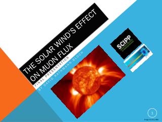
The Solar Wind’s Effect on Muon Flux. Final Presentation By David Rathmann -Bloch. Image Source: BBC. Abstract.

E N D
The Solar Wind’s Effect on Muon Flux Final Presentation By David Rathmann-Bloch Image Source: BBC
Abstract • This experiment sought to evaluate the impact of the solar wind on the amount of muonscoming in by correlating the rate of muon flux detected in a Quarknet 6000-series Scintillator detectorwith a) the natural day-night cycle an b) the dynamic solar wind data from NASA's SOHO satellite. • Using two different experimental setups (each running for 64 hours), the experimenter observed no statistically significant correlation between the day-night cycle and the rate of muon flux. He did, however, observe a seemingly statistically significant positive correlation between the muon flux and the real-time solar wind data; nevertheless, that correlation was neither linear nor completely supported by the data. On the setup with the detectors stacked atop one another and pointing directly up at the sky, a stronger visual correlation was observed (71% of data points within one standard deviation; 94% within two). When the Pearson Equation was used to find a correlation, it gave a value of about 0.44 (2 significant figures), which shows a mild positive correlation. On the setup with the detectors separated by a box and pointed toward the ecliptic, the visual correlation was not well shown (65% within one standard deviation; 88% within two). The Pearson value on the second data run showed a very, very weak negative correlation of -0.12. • Thus, this experiment showed no visible correlation between the day/night cycle and the muon flux. Using all four detectors stacked directly atop one another, it showed a mild positive correlation between the solar wind density and the measured muon flux. Using all four detectors, pointed toward the ecliptic, with a box in between them, the experiment showed no statistically significant correlation. Image Source: DeviantArt (users: Nightangel/Monoxism)
Focus Questions • How does the rate at which muons and other particles arrive change over time? • What does that demonstrate about the effects of the solar wind? • What significance does this have in a greater context? Image Source: Daniel Wilkinson
Background research • Experiments similar to this one have, indeed, been completed in the past. • “Measurements of the Cosmic Muon Flux with the Willi Detector as a Source of Information about Solar Events” (Bucharest, 2010) found that there was approximately a 5% increase in muons during the day. • “Solar Wind Effect on the MuonFlux at Sea Level” (Rio De Janeiro, 2005) found that “Forbush events” in which the sun ejects plasma, and the muon flux is decreased, are common. Thus, solar events can sometimes be negatively correlated with muon flux. Image Source: Creative Commons (User: Originalwana)
Solar wind: A quotidian (Daily) pattern? • Initially, this experiment will compare muon flux during the day and at night. I will associate these day and night fluctuations with the solar wind by the following assumptions. • In some cases, it takes particles from the solar wind many days to reach the earth. • However, I think that those particles likely to affect my muon count will almost certainly be traveling closer to the speed of light; ergo, there will only be eight to ten minutes of delay between solar events and local events. • Furthermore, for those particles most likely to result in muon production (or for those most likely to interfere with muon flux), it is reasonable for me to assume that, during the night, the earth’s large mass will prevent them from reaching my detector. • Image Source: Zastavski.com
Hypothesis • When the experiment is run, slightly more muons will likely be detected during the day, because some of them come from the solar wind. During the night, the earth will probably shield the detectors from those muons, so the muon flux (rate of arrival) will decrease slightly. However, it’s also possible that the opposite will occur: more muons may be detected at night due to a decrease in solar wind modulation of the cosmic ray spectrum. Image Source: collidingparticles.com
Hypothesis (continued) • If the initial portion of my hypothesis (as well as my assumptions) is correct, a fair conclusion should be that the solar wind bolsters, rather than attenuates, the rate of muon flux. • If the first two components of my hypothesis are correct, I can conclude that the solar wind consists partially of particles that end up creating muons, because the modulation effect is well known and would reduce the rate of muon flux, were it the only variable in play. Image Source: collidingparticles.com
Experimental technique Overview • After plateauing the four scintillators connected to a Quarknet DAQ board, I measure the muon flux by looking at the times when all four detectors are triggered simultaneously (within 40 ns of each other). Image Source: Fermilab
Detailed setup, 1st experiment • 1) Without plugging the DAQ into a power source, connect all four scintillators’ data cables into the DAQ. Then, plug their power cables into the voltage regulator. • 2) Plug the voltage regulator cable into the DAQ. Then, plug a CAT5 cable into your GPS receiver and your DAQ’s GPS IN port. • 3) Plug the USB (type B) connector into the DAQ and into a PC. You may need to install the CP210x Serial-to-USB driver on your PC. • 4) Finally, after ensuring that each connection is tight, plug your DAQ into an electric outlet. • 5) Start hyperterminal on your PC, and set up a new connection. Call it COM-3, use the port “COM3” and set the Bits per second to 115200. Finally, set the flow control to XON/XOFF. • 6) Ensure that the scintillators are stacked on top of one another in order, and properly plateaued (see Quarknet’s Plateauing guidelines for more details). There should be no more than four centimeters between detectors, and they should be flat, facing up. • 7) Run a short test at 4 coincidences. You should get approximately 5-8 counts per second, or 400-600 per minute (WC 00 3F ; 0.770 V in daytime). • 8) Ensure other variables (time delay, threshold voltage, etc.) are set to their defaults for the Quarknet 6000 DAQ. • Image Source: NASA
Detailed procedure of both experiments • 1) Prepare experimental equipment, as discussed in previous slide (or, for second experiment, on slides eighteen and nineteen). • 2) Set up DAQ board to take data over a 24-hour (or longer) period. It should be counting four coincidences on all four stacked detectors (WC 00 3F via the COM/USB interface; http://quarknet.fnal.gov/toolkits/ati/det-user.pdffor assistance). • 3) Capture the text data using the Quarknet guidelines. • 4) After 64 hours, finish the data collection, following the Quarknet guidelines. Run a Flux analysis. • 5) From this raw data, make a more detailed result and propose an explanation (e.g., muon flux was 5% higher during the day, perhaps because some muons came from the solar wind). • 6) Attempt to identify trends in the data. Also, check to see if the data correlate with real-time measurements of the solar wind using a visual standard deviation test and a Pearson (PPMCC) statistical correlation test. • 7) Document findings, procedures, and potential sources of error. • Image Source: NASA
Image Source: Sydney Electrical Contractors Plateauing Data • To reduce noise and ensure the detectors’ functionality, I plateau the detectors by adjusting their voltage and comparing it to the count rate. Plateau occurs around 0.80 V
Preliminary resulTs After running the detector for five days, with all the scintillators stacked directly on top of one another, I receive the graph above.
Interpreting My preliminary results • What do these data tell us? • No discernible daily pattern. • Fluctuations are generally not terribly statistically significant, at least with a bin width of four hours (1-3 error bars) • Further investigation is needed! Peaks Irregular Curve Outlier!
Interpreting results (Continued) Visually, however, we can correlate our muon flux pattern (outlier omitted) to real-time solar wind data from NASA’s SOHO satellite! How does this impact our interpretation of the focus questions & hypothesis? • Ultimately, we can’t conclude that the day/night cycle has a direct impact on the rate of muon arrival (flux) • This probably denies our hypothesis. • Once again, further investigation is needed. Image Sources: NASA, NOAA
Notes on my data fit • Of course, this graph was not produced without a few statistical adjustments (see below). • With these adjustments, 23 of my 32 (71%) 2-hour averages appear to be within one standard deviation of the SOHO data. Seven are within two standard deviations. Only two lie outside two standard deviations. Proton density is measured logarithmically But muon flux’s y-axis is measured linearly, from a flux of 8100 to 8600 events/m2/minute. The scale is also offset by one hour, because these protons take longer to reach the earth than the satellite
Pearson test of statistical correlation • We can calculate the degree of similarity between the two data sets by comparing the expected correlation (none) with the observed correlation. An R-value substantially greater than zero means a positive correlation; an R-value substantially less than zero means a negative correlation. • = Equaion source: Wikipedia
Interpreting the pearsonValue Putting all of the data into the Pearson equation, I receive a value of approximately 0.44. For my sample size (thousands of points; only 32 bins), I think this means that there is a statistically significant correlation between the two data sets. Image Source: “Skbekas”
The initial assumptions I made when starting the experiment are probably incorrect! • I assumed that day and night variations in high-energy solar wind would be more important than changes in overall solar wind density. • By correlating my results with the measurements of the SOHO satellite, I can see that the proton density of the solar wind in space seems to predict changes in terrestrial muon flux. A paradigmatic shift in my Hypothesis Image Source: NASA
Altering the procedure • Experimental changes may add precision to my data and thus make it easier to confirm the observed trend in a second data run. • It’s possible that orienting the detectors directly toward the ecliptic will de-munge (reveal the true patterns in) the data. By placing the detectors further apart, and pointing them at the ecliptic (72 degrees in July), I’ll be able to reduce the solid angle of the sky and reduce the disparity in terms of units and scale between the two data sets. This may also increase my R-value from the PPMCC test, helping confirm my correlation; or, it could make a false correlation disappear. Image Source: collidingparticles.com
Experimental Setup, second edition Box height = 21 cm Top scintillator Central box to reduce solid angle Angle of 72 degrees to point toward ecliptic. Image Source: collidingparticles.com
Second Run resulTs After running the detector for three days, with all the scintillators stacked according to the 2nd Edition Experimental Setup, I receive the graph above. It also shows no day/night cycle.
Interpreting results – 2nd experiment How well do our data correlate this time? Flux Density Flux Speed Flux Temperature Image Sources: NASA, NOAA
Notes on my 2nd data fit • The data do not seem to support as strong a correlation this time. Visually, my adjusted data gives the following conclusions: 21 of my 32 (66%) 2-hour averages appear to be within one standard deviation of the SOHO data; seven are within two standard deviations; and four lie outside two standard deviations. • Once again, this graph was not produced without a few statistical adjustments (see below). Proton density is measured logarithmically (same scale as before) But muon flux’s y-axis is measured linearly, from a flux of 2600 to 2750 events/m2/minute. (Yes, the flux went down.) The scale is offset once again by one hour, because these protons take longer to reach the earth than the satellite
Pearson Test, 2nd Experiment • =on the data set gives us a value of about -0.12, which is not all that statistically significant for my sample size, and definitely does not indicate a positive correlation. It could indicate a very, very slight negative correlation. Image Source: “Skbekas”
A disparity between two techniques? • The second experiment (euphemistically) doesn’t look as well correlated as the first did. • It’s possible that the first result was unusual and that a re-run of the first experiment would not indicate a correlation with the solar wind density. • It’s also possible that the second half of the second experiment was atypical due to unexplained phenomena. • It’s possible that poorly controlled variables in the second experiment impacted the results. From a visual inspection, the experimental setup may have sagged by about 2 cm over time, which could have put the detectors out of alignment and caused the steady downward trend in flux during the second half of the data run. I wasn’t able to verify if that occurred or not. • In the second experiment, increasing the distance between detectors reduced the overall flux by about 2/3; it likely reduced the signal-to-noise ratio by that amount. Image Source: NASA
Further research • This experiment’s conclusion is not terribly strong: a correlation observed using one experimental technique disappeared when the technique was altered. If I had more time and resources, I would do more data runs using the first experimental setup to see if the correlation observed was a statistical blip or whether it was a consistent finding. Then, I would do more data runs using the second experimental setup (but perhaps one manufactured to greater precision) to see if I could verify the disparity between the two setups. Image Source: NASA
Conclusion • I cannot yet make a conclusion about whether the terrestrial muon flux is correlated with the solar wind density in space, because I found contradictory results. • I can conclude that there is no direct correlation between the terrestrial muon flux and the day/night cycle, at least as observed in this experiment.
Thanks for watching! • Special thanks to: • Stuart Briber • Vicki Johnson • Jason Nielsen • TanmayiSai • Brendan Wells • the speakers • & my fellow interns Image Source: DeviantArt(user: TrekkieTechie)