Download
1 / 72
730 likes | 963 Views
Covering Solar-Wind Charge-Exchange from Every Angle with Chandra. Brad Wargelin Chandra X-Ray Center Smithsonian Astrophysical Observatory. Heliospheric Solar Wind Charge Exchange. Charge Exchange: The Forgotten Atomic Physics. Outline. Astrophysical charge exchange

E N D
Covering Solar-Wind Charge-Exchange from Every Angle with Chandra Brad Wargelin Chandra X-Ray Center Smithsonian Astrophysical Observatory
Charge Exchange: The Forgotten Atomic Physics
Outline Astrophysical charge exchange • Solar wind charge exchange Charge exchange X-ray emission Solar Wind Charge Exchange (SWCX) X-rays • ROSAT • Geocoronal CX • Heliospheric CX • Soft X-Ray Background and SWCX SWCX in the Chandra Deep Field-South Future observations
Charge Exchange Charge exchange (CX) is the radiationless transfer of one (or more) electrons from a neutral atom or molecule to an ion. • Molecular cloud chemistry: O+ + H O + H+ (13.618,13.599 eV) • Solar wind proton-H CX: H+ + H H + H+ • Some SW protons (tied to B field) CX with neutral H from the ISM, particularly between the heliopause and bowshock, creating hot H atoms, or Energetic Neutral Atoms (ENAs).
Local Interstellar Cloud (partially neutral, 26 km/s) Hydrogen Wall
IBEX and ENA Imaging • Energetic Neutral Atoms (ENAs) no longer tied to B field. These can be “seen” by the Interstellar Boundary Explorer (IBEX) to image the CX interaction region.
Astrospheres and Mass Loss Rates • Excess blue-shifted/broadened Lyman-α absorption due to the hot atoms in the Hydrogen wall can be used to determine mass loss rates of other stars surrounded by partially neutral ISM (Wood, et al. 2001-2005). Top line = intrinsic stellar profile (modeled) Dashed = after ISM absorption Hashed = excess absorption vs other lines a Cen B Lya; Linsky & Wood (1996)
Ionization balance of metals in photoionized nebulae—CX cross sections are large and a tiny fraction of neutral H is all it takes to make CX more important than RR and DR (e.g., Dalgarno 1985, Ferland et al. 1997). Emission of 511-keV annihilation line in the GC via positronium formation (nearly 100%). Roughly half of the positronium is formed via CX with the rest from RR. (2g emission with opposite spins, 3g with same spin.) Churazov et al. (2005, 2011)
Charge Exchange X-Rays O8+ + H *O7++ H+ O7+ + H + hn Highly charged ions capture electrons into high-n levels (nmax ~ q3/4) that emit X-rays. CX is a semi-resonant process. During a collision, energy levels distort and overlap at “curve crossings.” Cross sections are large (few × 10-15 cm2). (13.6 eV) (35 eV)
CX X-Rays in Olden Times ASCA; Tanaka (2002) Idea dates back to 1970s: • Galactic Ridge X-rays from cosmic rays? (Silk & Steigman 1969) S Ar Ca Fe ASCA spectra of GC, Sgr, Sct with identical model curves (other than norm, NH, 6.4-keV line).
CX X-Rays in Olden Times Idea dates back to 1970s: • Galactic Ridge X-rays from cosmic rays? • No. • Watson (1976), • Bussard et al. (1978)… • Revnivtsev et al. (2006, 2007)
CX X-Rays in Olden Times Idea dates back to 1970s: • Galactic Ridge X-rays from cosmic rays? • X-ray lasers: population inversion in “hollow ions”
CX X-Rays in Olden Times Idea dates back to 1970s: • Galactic Ridge X-rays from cosmic rays? • X-ray lasers: population inversion in “hollow ions” • Tokamaks: plasma edges and neutral beam heating (e.g., Rice et al. 1986) Na10+ n=7-1 Wargelin et al. (1998)
CX X-Rays in Olden Times Idea dates back to 1970s: • Galactic Ridge X-rays from cosmic rays? • X-ray lasers: population inversion in “hollow ions” • Tokamaks: plasma edges and neutral beam heating • Supernova remnants (Wise & Sarazin 1989)
CX X-Rays in Olden Times Idea dates back to 1970s: • Galactic Ridge X-rays from cosmic rays? • X-ray lasers: population inversion in “hollow ions” • Tokamaks: plasma edges and neutral beam heating • Supernova remnants? Cygnus Loop; Katsuda et al. (2011)
CX X-Rays in Olden Times Idea dates back to 1970s: • Galactic Ridge X-rays from cosmic rays? • X-ray lasers: population inversion in “hollow ions” • Tokamaks: plasma edges and neutral beam heating • Supernova remnants? CX X-ray emission was known
Discovery of Solar Wind CX X-Rays Key events: • Comet Hyakutake, ROSAT (Lisse et al. 1996) • SWCX explanation (Cravens 1997): Highly charged ions in SW + neutral H2O, CO, CO2
SWCX X-ray Spectrum (for Slow Wind) Model CX spectrum (C,N,O) with 6 eV resolution Wargelin et al. (2004)
Discovery of Solar Wind CX X-Rays LINEAR S4 Key events: • Comet Hyakutake, ROSAT (Lisse et al. 1996) • SWCX explanation (Cravens 1997) • First CCD spectrum of comet, by Chandra (Lisse et al. 2000) C/1999 S4 (LINEAR) Chandra/Lisse 2000 Beiersdorfer et al. (2003)
Discovery of Solar Wind CX X-Rays LINEAR S4 Key events: • Comet Hyakutake, ROSAT (Lisse et al. 1996) • SWCX explanation (Cravens 1997) • First CCD spectrum of comet, by Chandra (Lisse et al. 2000) C/1999 S4 (LINEAR) Chandra/Lisse 2000 Two dozen comets and several planets to date by ROSAT, EUVE, BeppoSAX, Chandra, XMM, Swift, Suzaku. Meanwhile…… Beiersdorfer et al. (2003)
LTEs & Discovery of Geocoronal and Heliospheric Emission ROSAT All Sky Survey (RASS; 1990) revealed multi-orbit (“Long Term”) enhancements in the SXRB. Cravens, Robertson, & Snowden (2001): temporal correlations between counting rate and SW flux LTEs are from geo/helio SWCX fluctuations. ¼-keV band, Galactic coords; Snowden et al. (2009)
Geocoronal Emission Geocoronal emission = SWCX in Earth’s exosphere, outside the magnetosphere (R > 10RE).
Geocoronal Emission Robertson et al. (2006) Geocoronal emission = SWCX in Earth’s exosphere, outside the magnetosphere (R > 10RE). X-ray missions generally look out through the flanks.
Lunar X-Rays (on the Dark Side) are Geocoronal ROSAT, Schmitt 1990 Chandra, Wargelin et al. 2004
Moon, Chandra; Wargelin et al. (2004) HDF-N, XMM; Snowden et al. (2004)
Heliospheric Charge Exchange Solar wind + H/He from ISM 100-AU halo Heliospheric CX ~ 10x geocoronal CX Model heliospheric emission from CX with H. Axis units in AU. LIC is moving to the right. Robertson et al. AIP Proc. 719 (2004).
Heliospheric Emission--looking down on ecliptic plane More neutral H upwind He focussing cone downwind (AU) (AU) Pepino et al. (2004)
Slow vs Fast Solar Wind At solar max, wind is a mix of slow and fast at ~all latitudes. At solar min, wind is stratified, with slow wind near the ecliptic. The fast wind is much less ionized and produces less CX X-ray emission.
CX Emission at Solar Min--view from Ecliptic Plane Stratified wind: slow and highly ionized near ecliptic higher CX emissivity. Little emission in fast wind. AU Pepino et al. (2004) AU
SXRB emission components: Absorbed extragalactic (~power law) Absorbed thermal Galactic Halo emission Unabsorbed thermal from Local Bubble Heliospheric and geocoronal SWCX The Soft X-Ray Background (SXRB) How much emission is from CX vs the Local Bubble? The answer strongly affects our models of the LB.
Modeling CX Emission • Need to know • H and He distributions • SW composition and density all along line of sight (LOS) • State-specific CX cross sections for all ions (and neutrals) as f(v) • Radiative decay paths and line yields Local SW measured by ACE
Living in a Fog We can try to observationally separate SWCX emission from cosmic components with differential measurements: • Spatially (using dark clouds to block distant emission) • Spectrally (some day, with high-resolution nondispersive detectors) • Temporal changes (periods of hours to Solar Cycle) • Observation geometry
The Chandra Deep Field-South 4 Msec of observations: • 3 in Oct, Nov 1999 (-110 C) • 9 in May, Jun, Dec 2000 • 12 in Sep-Nov 2007 • 31 in Mar-Aug 2010 RA,Dec 3:32:28, -27:48:30 Gal l,b 223.6, -54.4 Ecl lat,lon 41.1, -45.2 The CDFS is the only X-ray deep field conducted during Solar Max and Min and it has the greatest orbital coverage.
LOS is 45 down, into page. 2000 0.8 Ms in 2000 (solar max) 1.0 Ms in 2007 (solar min) 2.0 Ms in 2010 (solar min) J. Slavin
In 2000, there is slow wind all along the LOS and most observations are from within the He cone. From within the He cone, CX intensity is higher and more of the emission is from nearby, where SW conditions are measured.
In 2007, SW is stratified, LOS through fast wind, observations all outside He cone, looking downwind.
Expectations for observed SXRB in 2000 vs 2007: • Higher baseline level • More variability • Closer correlation with ACE-measured SW ion flux
Compare O emission vs average ACE/SWICS O7+ flux Many thanks to the ACE/SWICS team for their public data!
2000: Higher SXRB Variable Correlated with local SW 2007: Lower SXRB Nearly constant Little correlation with SW
The goal is to accurately model and remove SWCX emission and obtain the true cosmic background. ?
The Future • High-resolution spectra from microcalorimeters will help immensely. Astro-H launch in 2014 (E ~ 5 eV) . • CX spectra differ from collisional: enhanced high-n Lyman, He-like f... • Explore the 1/4-keV band (where ROSAT LTEs are strongest) • 500 km/sec E=1 eV at 600 eV
100 s of SXRB from XQC rocket flight vs thermal model (McCammon et al. 2002)
CX Spectra High-n levels are preferentially populated.
CX Spectra High-n levels are preferentially populated. • H-like: enhanced high-n H-like Fe (with N2 in EBIT)
CX Spectra High-n levels are preferentially populated. • H-like: enhanced high-n • He-like: enhanced triplet f and i EIE at 15 keV He-like Fe CX with N2 10 eV/amu Wargelin et al. (2008)
Astrospheric Charge Exchange CX must also occur around other stars with highly ionized winds (G,K,M) residing inside clouds with neutral gas (LIC, G). Imaging + spectra yields: • Mass-loss rate • Local nneutral • Wind velocity and composition • Astrosphere geometry Coronal emission is ~104x brighter, though. Need very large collecting area, good spatial and spectra resolution.
Reviews “Charge Transfer Reactions” Dennerl, Space Sci. Rev. (2010) Astrophysical examples and broad historical review “EBIT charge-exchange measurements and astrophysical applications,” Wargelin et al., Canadian J. Physics (2008) Astrophysical examples and lab spectra/atomic physics