Section 6.1
Section 6.1. Exploring Quantitative Data. Quantitative vs. Categorical Variables. Categorical Labels for which arithmetic does not make sense. Sex , ethnicity, eye color … Quantitative You can add, subtract, etc. with the values. Age , height, weight, distance, time… .


Section 6.1
E N D
Presentation Transcript
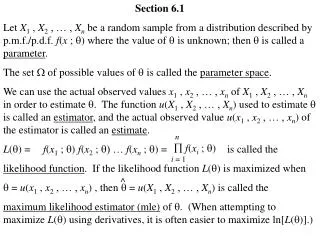
Section 6.1 Exploring Quantitative Data
Quantitative vs. Categorical Variables • Categorical • Labels for which arithmetic does not make sense. • Sex, ethnicity, eye color… • Quantitative • You can add, subtract, etc. with the values. • Age, height, weight, distance, time…
Visualizing Single Variable Data Categorical Quantitative Dot Plot Bar Graph
Comparing Two Groups Graphically • Categorical • Quantitative
Notation Check Statistics • (x-bar) Sample Average or Mean • (p-hat) Sample Proportion Parameters • (mu) Population Average or Mean • (pi) Population Proportion or Probability Statistics summarize a sample and parameters summarize a population
Exploration 6.1 • Haircut Prices Before After
Section 6.2 Simulation-Based Approach for Comparing Two Means
Comparison to Proportions • We will be comparing means, much the same way we compared two proportions using randomization techniques with cards and an applet. • The difference here is that instead of two categorical variables, our explanatory variable will be categorical and the response variable will be quantitative variable.
Bicycling to Work Example 6.2
Bicycling to Work • Does bicycle weight affect commute time? • British Medical Journal (2010) presented the results of a randomized experiment conducted by Jeremy Groves. • Groves wanted to know if bicycle weight affected his commute to work. • For 56 days (January to July) Groves tossed a coin to decide if he would bike the 27 miles to work on his carbon frame bike (20.9lbs) or steel frame bicycle (29.75lbs). • He recorded the commute time for each trip.
Bicycling to Work • What are the observational units? • Each trip to work on the 56 different days. • What are the explanatory and response variables? • Explanatory is which bike Groves rode (categorical – binary) • Response variable is his commute time (quantitative)
Bicycling to Work • Null hypothesis:There is no association between which bike is used and commute time • Commute time is not affected by which bike is used. • Alternative hypothesis:There is an association between which bike is used and commute time • Commute time is affected by which bike is used.
Bicycling to Work • In chapter 5 we used the difference in proportionsof “successes” between the two groups. • Now we will compare the difference in averagesbetween the two groups. • The parameters of interest are: • µcarbon = Long term average commute time with carbon frame bike • µsteel= Long term average commute time with steel frame bike.
Bicycling to Work • Mu (µ) is the parameter for population mean. • Using the symbols µcarbon and µsteel, restate the hypotheses: • H0:µcarbon= µsteel OR µcarbon– µsteel = 0 • Ha:µcarbon≠ µsteelOR µcarbon– µsteel ≠ 0
Bicycling to Work Remember • The hypotheses are about the association between commute time and bike used, not just his 56 trips. • Hypotheses are always about populations or processes, not the sample data.
Bicycling to Work • Results
Bicycling to Work • The sample average and variability for commute time was higher for the carbon frame bike • Does this indicate a tendency? • Or is it just random assignment and traffic was heavier on those days?
Bicycling to Work • Is it possible to get a difference of 0.53 minutes if commute time isn’t affected by the bike used? • The same type of question was asked in Chapter 5 for categorical response variables. • The same answer. Yes it’s possible, how likely though?
Bicycling to Work • The 3S Strategy Statistic: • Choose a statistic: • The observed difference in average commute times carbon – steel= 108.34 - 107.81 = 0.53 minutes
Bicycling to Work Simulation: • We can simulate this study with index cards. • Write all 56 times on 56 cards. • Shuffle all 56 cards and randomly redistribute into two stacks: • One with 26 cards (representing the times for the carbon-frame bike) • Another 30 cards (representing the times for the steel-frame bike)
Bicycling to Work • Shuffling assumes the null hypothesis of no association between commute time and bike • Calculate the difference in the average times between the two stacks of cards. • Repeating this many times develops a null distribution • Let’s see how this process is sped up with the two means or multiple means applets.
Bicycling to Work • What does this p-value mean? • If mean commute times for the bikes are the same, and we repeated random assignment of the lighter bike to 26 days and the heavier to 30 days, a difference as extreme as 0.53 minutes or more would occur in about 70.5% of the repetitions. • Therefore, we don’t have evidence that the commute times for the two bikes will differ in the long run.
Bicycling to Work • Have we proven that the bike Groves chooses is not associated with commute time? (Can we conclude the null?) • No, a large p-value is not “strong evidence that the null hypothesis is true.” • It suggests that the null hypothesis is plausible • There could be long-term difference just like we saw, but it is just very small.
Bicycling to Work • Let’s use the 2SD Method to generate a confidence interval for the long-run difference in average commuting time. • Sample difference in means ± 2⨯SD of the simulated null distribution • Our standard deviation for the null distribution was 1.49 • 0.53 ± 2(1.49)= 0.53 ± 2.98 • -2.45 to 3.51. • What does this mean? (next page)
Bicycling to Work • We are 95% confident that the true difference (carbon – steel) in average commuting times is between -2.45 and 3.51 minutes. Carbon frame bike is between 2.45 minutes faster and 3.51 minutes slower than the steel frame bike. • Does it make sense that the interval contains 0 based on our p-value?
Bicycling to Work Scope of conclusions • Can we generalize our conclusion to a larger population? • Two Key questions: • Was the sample randomly obtained from a larger population? • Were the observational units randomly assigned to treatments?
Bicycling to Work • Was the sample randomly obtained from a larger population? • No, Groves commuted on consecutive days which didn’t include all seasons. • Were the observational units randomly assigned to treatments? • Yes, he flipped a coin for the bike • We can draw cause-and-effect conclusions
Bicycling to Work • We can’t generalize beyond Groves and his 2 bikes. • A limitation is that this study is that it’s not double-blind • The researcher and the subject (which happened to be the same person) were not blind to which treatment was being used. • Perhaps Groves likes his old bike and wanted to show it was just as good as the new carbon-frame bike for commuting to work.
Exploration • Exploration 6.2: Lingering Effects of Sleep Deprivation
Section 6.3: Comparing Two Averages: Theory-Based Methods • Just as we’ve seen with one proportion, and two proportions there are simulation-based methods to conduct tests of significance and theory-based ones. • Theory-based methods use some distribution to model our null distribution. • With the proportions, this is a normal distribution. • With means we will use a t-distribution.
T-distributions • t-distributions have a similar bell-shape to that of normal distributions. • For small sample sizes, the t-distributions we will use to model our null hypotheses are shorter and wider than normal distributions with the same mean and standard deviation. • As the sample size increases, the curve comes closer and closer to a normal curve.
Sleep Deprivation Distributions from previous section Bike Times Bell-shaped. Centered at 0. Different Standard Deviations. Bike Times(1.50) Sleep Deprivation(6.52)
Distributions • Graphs centered at 0 • The graphs were generated based on the null hypothesis that the population means of the groups are the same. • Not all results are 0 due to sample to sample variability. • Variability (Standard Deviation) depends on: • The amount of variability in our samples. • The samples size. • This variability can be predicted.
Distributions • Will the bell-shape always appear? • No. It appears when the sample size is large enough or if the population distributions are bell-shaped. • Validity Conditions (We can use theory-based techniques if either of the following is true.) • Sample sizes of at least 20 in each group. • The distributions of each response variable is bell-shaped.
Breastfeeding and Intelligence Example 6.3
Breastfeeding and Intelligence • A study in Pediatrics (1999) examined if children who were breastfed during infancy differed from bottle-fed. • Involved 323 white children recruited at birth in 1980-81 from four Western Michigan hospitals. • Researchers deemed the participants as representative of the community in social class, maternal education, age, marital status, and sex of infant. • Children were followed-up at age 4 and assessed using The General Cognitive Index (GCI) • A measure of the child’s intellectual functioning • Also recorded if the child had been breastfed during infancy.
Breastfeeding and Intelligence • Explanatory and response variables. • Explanatory variable: If the baby was breastfed. (Categorical) • Response variable: Baby’s GCI measure at age 4. (Quantitative) • Is this experimental or observational? • Can cause-and-effect conclusions be drawn in this study?
Breastfeeding and Intelligence • Null hypothesis:There is no association between breastfeeding during infancy and GCI at age 4. • Alternative hypothesis:There is an association between breastfeeding during infancy and GCI at age 4.
Breastfeeding and Intelligence • µbreastfed = Average GCI at age 4 for breastfed children • µnot = Average GCI at age 4 for children not breastfed • H0: µbreastfed = µnot (µbreastfed– µnot = 0) • Ha: µbreastfed ≠ µnot (µbreastfed– µnot ≠ 0)
Breastfeeding and Intelligence The difference in means was 4.4. • If breastfeeding is not associated with GCI at age 4: • Is it possible a difference this large could happen by chance alone? Yes • Is it plausible (believable, fairly likely) a difference this large could happen by chance alone? Let’s find outusing the multiple means applet.
Breastfeeding and Intelligence Meaning of the p-value: • If breastfeeding were not associated with GCI at age 4 (our true null) the probability of observing a difference of 4.4 or more or -4.4 or less just by chance is 0.01. Since the sample sizes are considered large enough (n1= 237, n2= 85), we can the theory-based approach to find the p-value.
Breastfeeding and Intelligence • Again we see we have strong evidence against the null hypothesis and can conclude there is an association between breastfeeding and intelligence. • In fact we can conclude that breastfed babies have higher average GCI scores at age 4. • We can see this in both the small p-value (0.015) and the confidence interval that says the mean GCI for breastfed babies is 0.87 to 7.93 points higher than that for non-breastfed babies.
Breastfeeding and Intelligence • To what larger population(s) would you be comfortable generalizing these results? • The participants were all white children born in Western Michigan. • This limits the population to whom we can generalize these results.
Breastfeeding and Intelligence • Can you conclude that breastfeeding improves average GCI at age 4? • No. The study was not a randomized experiment. • Can’t conclude a cause-and-effect relationship. • There might be alternative explanations for the significant difference in average GCI values. • Maybe better educated mothers are more likely to breastfeed their children • Maybe mothers that breastfeed spend more time with their children and interact with them more. • There could be many confounding variables.
Breastfeeding and Intelligence • Could you design a study that allows drawing a cause-and-effect conclusion? • We would have to run an experiment using random assignment to determine which mothers breastfeed and which would not. (Though it still can’t be double-blind.) • Random assignment balances out all other variables. • Is it feasible/ethical to conduct such a study? • No. A personal decision can’t be imposed on mothers.
Strength of Evidence • We already know: • As sample size increases, the strength of evidence increases. • Just as with proportions, as the sample means move farther apart, the strength of evidence increases.
More Strength of Evidence • We now have standard deviation • If the means are the same distance apart, but the standard deviations are quite different. Which gives stronger evidence against the null?