Download
1 / 12
130 likes | 233 Views
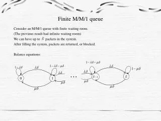
Consider the M/M/1 queue. Arrival process: Poi( t) Service distribution: Poi(t) One server, infinite queue length possible Prob(arrival in small interval h ) = h Prob(service completed in small interval h ) = h We know P 0 , but what else can we say, e.g. P 1 , P 2 etc.

E N D
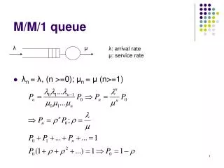
Consider the M/M/1 queue • Arrival process: Poi(t) • Service distribution: Poi(t) • One server, infinite queue length possible • Prob(arrival in small interval h) = h • Prob(service completed in small interval h) = h • We know P0 , but what else can we say, e.g. P1 , P2 etc
Possible states (sizes) of a queue ... State 0 1 2 n-1 n n+1 • Pn is how often system is in state n ( n jobs in queue) • M/M/1 queue: Consider small interval of time h • P(Jump from state n-1 to n) = P(arrival) = h (flow from n-1 to n) • P(Jump from state n to n-1) = P(departure) = h (flow from n to n-1) • Flow between states must be balanced. If not …. • Let’s look at states 1 and 0. What is the flow between them ?
Flow equations for M/M/1 queue • In steady state inflows = outflows • Flow into state 0 = P1 • Flow out of 0 = P0 • For balance: P0 = P1 P1 = (/ ) P0 = P0 = (1-) • Flow into state 1 = P0 + P2 • Flow out of 1 = P1 + P1 • For balance: P0 + P2 = P1 + P1
Steadystate probabilities • We have P0 = 1- , P1 = (1-) P2 = (+ ) P1 -P0 P2 = (1 + ) (1-) - (1-) = 2 (1-) • Balance equation for state n • Pn-1 + Pn+1 = Pn + Pn • By induction, the solution is: Pn = n (1-) • Check that this is a valid probability distr. • P0 + P1 +… =
Results for M/M/1 • P( n jobs in system) = Pn = n (1-) • P(at least m jobs in system)
Performance of M/M/1 • N = E(no. in system) = • R =
Performance depends on As 1, N e.g. =0.8, N =4 =0.9, N =9 =0.95, N =17 =0.90, N =99 R (utilisation)
Bound of utilisation • = (/ ) is called the utilisation or traffic intensity of the queueing system • determines the performance of an M/M/1 queue • as 1, N • So, for steady state queue, we need < 1 • i.e. < , or arrival rate is slower than service rate
Other queueing disciplines Q: Are results affected by queue disciplines ? A: Not as long as queue discipline does not make explicit use of job lengths, i.e. N = / (1-) for M/M/1 FCFS, LCFS, round robin, least attained service first but N / (1-) for SJF
Example of M/M/1 • Randomly arriving messages of variable length are transmitted over a channel (waiting mess. stored in buffer) • Avg message length = 128 octets • Line bit rate = 4800 bits per second. • Message arrival rate = 7500 per hour. (a) What is the probability of the buffer being empty? (b) What is the average no. of messages in the system? (c) What is the average number of bits in the buffer? (d) What is the average delay of a message?
FDMA for mobile phone network • N streams single communication line • stream arrival rate = packets per second • average transmission time for stream= 1/
Performance of FDMA • What is avg. no. in system ? • What is avg. delay ? • How does it compare to single channel M/M/1 (statistical multiplexing) ?