Download
1 / 28
280 likes | 417 Views
Explore the optimality of scheduling disciplines in M/G/1 queue using Gittins Index. Investigate conditions for optimality of FCFS and FB. Examine service time distribution classes and new optimality results.

E N D
On the Gittins indexin the M/G/1 queue Samuli Aalto (TKK) in cooperation with Urtzi Ayesta (LAAS-CNRS) Rhonda Righter (UC Berkeley)
Fundamental question • It is well known that … • … in the M/G/1 queue • … among the non-anticipating scheduling disciplines • … the optimal discipline is • FCFS if the service times are NBUE • FB if the service times are DHR • So, these conditions are sufficient for the optimality of FCFS and FB, respectively. But, … Are the conditions necessary?
Outline • Service time distribution classes • Known optimality results • Gittins index • Gittins index and service time distribution classes • Gittins index policy • New optimality results
Queueing model (1) • M/G/1 queue • Poisson arrivals with rate l • IID service times S with a general distribution • single server • Service time distribution: • Density function: • Hazard rate:
Queueing model (2) • Remaining service time distribution: • Mean remaining service time: • H-function:
NBUE NWUE DMRL IMRL IHR DHR Service time distribution classes (1) • Service times are • IHR [DHR] if h(x) is increasing [decreasing] • DMRL [IMRL] if H(x) is increasing [decreasing] • NBUE [NWUE] if H(0) £[³]H(x) • It is known that • IHR Ì DMRL Ì NBUE and DHR Ì IMRL Ì NWUE
NBUE NWUE DMRL IMRL IHR DHR Service time distribution classes (2) • IHR = Increasing Hazard Rate • DMRL = Decreasing Mean Residual Lifetime • NBUE = New Better than Used in Expectation • DHR = Decreasing Hazard Rate • IMRL = Increasing Mean Residual Lifetime • NWUE = New Worse than Used in Expectation
Outline • Service time distribution classes • Known optimality results • Gittins index • Gittins index and service time distribution classes • Gittins index policy • New optimality results
Scheduling/queueing/service disciplines • Anticipating: • SRPT = Shortest-Remaining-Processing-Time • strict priority according to the remaining service • Non-anticipating: • FCFS = First-Come-First-Served • service in the arrival order • FB = Foreground-Background • strict priority according to the attained service • a.k.a. LAS = Least-Attained-Service
NWUE NBUE DMRL IMRL IHR DHR Known optimality results • Among all scheduling disciplines, • SRPT is optimal(minimizing the queue length pathwise); Schrage (1968) • Among the non-anticipatingscheduling disciplines, • FCFS isoptimal for NBUE service times (minimizing the mean queue length); Righter, Shanthikumar and Yamazaki (1990) • FB isoptimal for DHR service times (minimizing the queue length stochastically); Righter and Shanthikumar (1989)
Our objective • We will show that … • … among the non-anticipatingscheduling disciplines • FCFS isoptimal only for NBUE service times • FB isoptimal only for DHR service times • In other words, we will show that … • For that, we need Yes, the conditions are necessary. The Gittins Index
Outline • Service time distribution classes • Known optimality results • Gittins index • Gittins index and service time distribution classes • Gittins index policy • New optimality results
Gittins index • Efficiency function (J-function): • Gittins index for a customer with attained service a: • Optimal (individual) service quota:
Example Pareto service time distribution starting from 1 k= 1 D*(0)= 3.732
Basic properties (1) • Partial derivative w.r.t. to D: • Lemma: • If D*(a) <¥ and h(x) is continuous, then
Basic properties (2) • Lemma: • Corollary: • Lemma: • Corollary:
Outline • Service time distribution classes • Known optimality results • Gittins index • Gittins index and service time distribution classes • Gittins index policy • New optimality results
DHR [IHR] service times • Lemma: • Proof: • Corollary: • If the service times are DHR [IHR], then J(a,D) is decreasing [increasing] w.r.t. to D for all a, D. • Corollary: • If the service times are DHR [IHR], then G(a)=h(a) [H(a)] for all a.
DHR service times • Proposition: • (i) The service times are DHR if and only if (ii) G(a) is decreasing for all a. • In this case, G(a)=h(a) for all a. • Proof: • (i) Þ (ii): Corollary in slide 18 • (ii) Þ (i): Corollary in slide 16
IMRL [DMRL] and NWUE [NBUE] service times • Lemma: • Proof: • Corollaries: • The service times are IMRL [DMRL] if and only if J(a,¥)£ [³] J(a,D) for all a, D. • The service times are NWUE [NBUE] if and only if J(0,¥)£ [³] J(0,D) for all D.
DMRL and NBUE service times • Proposition: • (i) The service times are DMRL if and only if (ii) G(a) is increasing for all a if and only if (iii) G(a)=H(a) for all a. • (i) The service times are NBUE if and only if (ii) G(a)³G(0) for all a if and only if (iii) G(0)=H(0). • Proof: • (i) Û (iii) Þ (ii): Corollary in slide 20 • (ii) Þ (i): Corollary/Lemma in slide 16
Outline • Service time distribution classes • Known optimality results • Gittins index • Gittins index and service time distribution classes • Gittins index policy • New optimality results
Gittins index policy • Definition [Gittins (1989)]: • Gittins index policy gives service to the job i with the highest Gittins index Gi(ai). • Theorem [Gittins (1989), Yashkov (1992)]: • Among the non-anticipating disciplines,Gittins index policy minimizes the mean queue length in the M/G/1 queue (with possibly multiple job classes) • Observations: • FB is a Gittins index policy if and only if G(a) is decreasing for all a. • FCFS (or any other non-preemptive policy) is a Gittins index policy if and only if G(a)³G(0) for all a.
Outline • Service time distribution classes • Known optimality results • Gittins index • Gittins index and service time distribution classes • Gittins index policy • New optimality results
Single job class (1) • Theorem: • FB minimizes stochastically the queue length if and only if the service times are DHR. • Proof: • Theorem in slide 23 and Proposition in slide 19 together with Righter, Shanthikumar and Yamazaki (1990). • Theorem: • FCFS minimizes the mean queue length if and only if the service times are NBUE. • Proof: • Theorem in slide 23 and Proposition in slide 21.
Single job class (2) • Additional assumption: • arriving jobs have already attained a random amount of service elsewhere • Theorem: • FB = LAS minimizes the mean queue length if and only if the service times are DHR. • Definition: • MAS (Most-Attained-Service) gives service to the job i with the highest hazard rate hi(ai). • Theorem: • MAS minimizes the mean queue length if and only if the service times are DMRL.
Multiple job classes • Additional assumption: • arriving jobs have already attained a random amount of service elsewhere • Definition: • HHR (Highest-Hazard-Rate) gives service to the job i with the highest hazard rate hi(ai). • Theorem: • If all service time distributions are DHR, then HHR minimizes the mean queue length • Theorem: • If all service time distributions are DMRL, then SERPT minimizes the mean queue length