COAS-CIOSS Coastal Ocean Modeling Activities

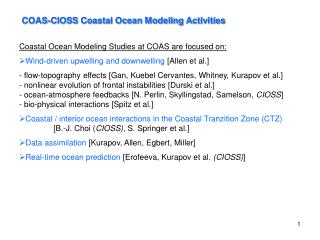
1. COAS-CIOSS Coastal Ocean Modeling Activities • Coastal Ocean Modeling Studies at COAS are focused on: • Wind-driven upwelling and downwelling [Allen et al.] • flow-topography effects [Gan, Kuebel Cervantes, Whitney, Kurapov et al.] • nonlinear evolution of frontal instabilities [Durski et al.] • ocean-atmosphere feedbacks [N. Perlin, Skyllingstad, Samelson, CIOSS] • bio-physical interactions [Spitz et al.] • Coastal / interior ocean interactions in the Coastal Tranzition Zone (CTZ) [B.-J. Choi (CIOSS), S. Springer et al.] • Data assimilation [Kurapov, Allen, Egbert, Miller] • Real-time ocean prediction [Erofeeva, Kurapov et al. (CIOSS)]

2. How does coastal ocean modeling help address CIOSS goals? • Dynamical interpretation of physical features apparent in satellite data (on the shelf and in the coastal transition zone) • Assimilation of satellite data, together with other data (providing dynamically based interpolation and mapping of the satellite data; filling gaps in space and time) • Analysis of physical models, integrated with observations, • - to improve scientific understanding of the ocean dynamics, and • - to predict the ocean dynamics

3. Coastal Ocean Dynamics off Oregon: Movie: surface T and tracers COAST Observing System, summer 2001 HF radars (Kosro) Moorings (ADP, T, S: Levine, Kosro, Boyd) Model:space-time continuoussolutions (velocity, T, S, turbulence quantities) (development of upwelling 12-22 June 2001, Princeton Ocean Model solution constrained by assimilation of COAST data)

4. Topographic effects [Kurapov et al., JPO, 2005]: On the mid-shelf, bottom mixed layer thickness is small at 45N, large at 44.4N in response to upwelling dB at 45N, H=98 m dB east of Stonewall Bank Turbulent KE in response to the upwelling event (day 170, 2001): Depth, 0 – 100 m At 45N At 44.4N 44.4N: As a result of bottom Ekman transport convergence, thinner surface BL, thicker bottom BL lon, W

5. Coupled Ocean-Atmosphere Modeling (N. Perlin, Skyllingstad, Samelson, with support from CIOSS and ONR): Accurate representations of coastal upwelling processes must include ocean-atmosphere interactions on short temporal and horizontal scales Effect of coupling on atmos. eddy visc. … COAMPS: wind, heat cold water ROMS: upwelling response (T) Initial value problem: run from rest for 72 h heat flux… wind stress [N. Perlin et al. JPO, submitted]

6. Dynamical coupling of the coastal ocean and California Current System (CCS) flows through the Coastal Tranzition Zone (CTZ) [B.-J. Choi (GLOBEC-NOAA, CIOSS), S. Springer (NOPP)] -Unstable, separating coastal flows feed into the CCS - Mesoscale eddies (CCS) affect variability in the coastal waters SSH (5/31/02): NCOM ROMS, NCOM • Nesting: • 9 km NCOM-CCS • Atm. forcing: COAMPS (16-km) • [J. Kindle (NRL)] • 3 km ROMS-CTZ • Open boundary conditions: appropriate for advective currents, coastal trapped waves, tides, Rossby waves, Columbia R. Can nesting improve the prediction of coastal currents? Can data assimilation help? -0.1 m 0.3 0.1

7. ROMS, NCOM NCOM SST (5/31/02): higher spatial variability in ROMS SST Surface Salinity: inclusion of Columbia R. in ROMS

8. Model-data comparisons: NCOM vs. alongtrack SSH altimetry Demeaned alongtrack SSH: T/P, NCOM 8 SSH RMS diff. (NCOM – Altim.), 2002 (cm) 4 0 1 SSH correlation (NCOM, Altim.), 2002 -0.5 0 -130 -128 -126 -124 longitude along satellite track -5 cm 40 Even though NCOM-CCS assimilates SSH using “nudging”, the data are not fit particularly well in the CTZ Room for improvement: assimilate alongtrack SSH, together with other obs. in the CTZ domain model

9. Data assimilation (DA) [Kurapov, Allen, Egbert, Miller, ONR] • Approach: • complicated, fully-nonlinear model + simple DA • simplified models + rigorous variational DA • Merger of approaches: nonlinear models + variational DA • Princeton OM + sequential Optimal Interpolation: assimilate HF radar (Oke et al. JGR 2002), moored velocity data (Kurapov et al. 2005abc) • Assimilation of moored ADP data: • improves model accuracy at a distance of 90 km in the alongshore dir. • improves prediction of T, S, SSH near coast, near-bottom turbulent dissipation

10. Variational DA: fit the model solution to the observations over a given time interval (by correcting errors in the inputs) Minimize the penalty function: J(u) = || model error ||2 + || obs. error ||2 Obtain information on the source of model error Utilize (compute) state-dependent model error covariance Assimilate observations (incl. satellite SSH, SST, HF radar) w/out pre-processing the observations into maps Variational DA: utilizes tangent linear and adjoint models, algorithmically complicated, computationally challenging Our path: representer-based optimization (following methodology developed by Bennett, Egbert, et al.) The nonlinear optimization problem is approached as a series of linearized problems. Each linearized problem: search for the solution correction in a relatively small subspace spanned by K representer solutions, where K is the number of observations (still, no need to compute all the representers)

11. Tests of the representer-based method (with the shallow-water model, describing flows in the near-shore surf zone): - assimilation in presence of instabilities, intrinsic eddy interactions - correction of forcing, open boundary conditions Equilib. shear wave regime (T=60 min) More irregular regime (T=5 min) True solution (shown is vorticity) Unsteady solution in response to steady forcing (Prior = 0) • DA solution: • assimilate time series of z, u, v at 32 pnts • correct IC, forcing Click on frame to play movie (left for 60 min, right for 5 min).

12. This looks way too good… somebody must be cheating… Real-time Oregon coastal simulation system (Erofeeva, Kurapov, Samelson, Egbert, CIOSS) ROMS (Dx = 2 km), forced with 3-day atmospheric NAM forecast: daily update Model data comparisons: SSH, SST (incl. monthly climatologies), HF radar data forecast (5/11/06) HF radar (Kosro) Additional QC: coordinated with the NOAA-funded OrCOOS pilot project (J. Barth, R. K. Shearman)

13. SUMMARY: • 1. Research involving coastal ocean modeling has been focused on flow/topography, ocean/atmosphere, CCS/shelf flow interactions. • 2.Variational DA has the potential of providing new versatile tools for synthesis of satellite, in-situ and land-based HF radar observations. • 3. Work to advance the real-time Oregon Coastal Simulation System will be leveraged by efforts on ongoing GLOBEC, NOPP, and ONR research projects • improved ROMS configuration • DA (alongtrack SSH, HF radar) • 4. The real-time modeling system will become an integral part of the emerging OrCOOS, facilitating interactions within COAS research community