Download
1 / 58
580 likes | 604 Views
This course provides an introduction to various mathematical concepts and tools for analyzing complex systems, covering topics such as iterative maps, stochastic systems, information theory, and more.

E N D
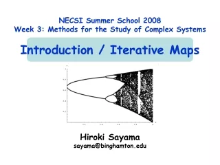
NECSI Summer School 2008Week 3: Methods for the Study of Complex SystemsIntroduction / Iterative Maps Hiroki Sayama sayama@binghamton.edu
Course objective • To provide an introduction to a variety of mathematical concepts and tools for analysis of complex systems • Textbook: Bar-Yam, Y. “Dynamics of Complex Systems” (Perseus Books/Westview Press, 1997)
Topics to be covered • Iterative maps • Stochastic systems • Information theory • Computation theory • Dynamical systems and phase space • Analytical tools for dynamical systems • PDEs and reaction-diffusion systems • Cellular automata • Thermodynamics and statistical mechanics • Stochastic fields and mean-field approximation • Monte Carlo simulations • Scaling, fractals and renormalization
Online resource • Course slides for the first two days are available at: http://coco.binghamton.edu/NECSI/ Login name: necsi Password: com3sysB
Course structure • Monday ~ Thursday • 9:00am~5:00pm: Lectures, discussions • 6:00pm~8:00pm: Group projects • Friday • 9:00am~12:00pm: Presentations (+ optional final exam)
Group projects • Presentation (~15 min.) + 5-page paper • Option 1: Original research • Conduct mathematical analysis of a model of complex systems (either existing or original) and report your findings • Option 2: Teaching analytical methods • Select some analytical method that is not covered in the classes, prepare teaching materials (including illustrative examples and questions) and deliver a lecture • Option 3: Problem sets (for individuals) • Go through several problems selected from different sections in textbook, write out your work and hand it in (presentation waived in this case)
Examples of complex systems • Chemical networks • Gene networks • Organisms • Physiologies • Brains • Ecosystems • Economies • Societies • Internet
Several characteristics of complex systems • Networks of many components • Nonlinear interactions • Self-organization • Structure/behavior that is neither regular nor random • Emergent behavior
Four approaches to complexity Nonlinear Dynamics Complexity = No closed-form solution, Chaos Information Complexity = Length of description, Entropy Computation Complexity = Computational time/space, Algorithmic complexity Collective Behavior Complexity = Multi-scale patterns, Emergence
Dynamical systems theory • Considers how systems autonomously change along time • Ranges from Newtonian mechanics to modern nonlinear dynamics theories • Thinks about underlying dynamical mechanisms, not just static properties of observations • Forms the theoretical basis for most of complex systems studies
What is a dynamical system? • A system whose state is uniquely specified by a finite set of variables and whose behavior is uniquely determined by predetermined rules • Simple population growth • Simple pendulum swinging • Motion of celestial bodies • Behavior of two “rational” agents in a negotiation game
Mathematical formulations of dynamical systems • Discrete-time model: xt = F(xt-1, t) • Continuous-time model: (differential equations) dx/dt = F(x, t) xt: State variable of the system at time t • May take “scalar” or “vector” value F: Some function that determines the rule that the system’s behavior will obey (difference/recurrence equations; iterative maps)
Difference equation and time series • Difference equation xt = F(xt-1, t) produces series of values of variable x starting with initial conditionx0: { x0, x1, x2, x3, … } “time series” • A prediction made by the above model (to be compared to experimental data)
Linear vs. nonlinear • Linear: • Right hand side is just a first-order polynomial of variables xt = a xt-1 + b xt-2 + c xt-3 … • Nonlinear: • Anything else xt = a xt-1 + b xt-22 + c xt-1 xt-3 …
Single-variable vs. multi-variable • Single-variable (univariate): • Just one equation given for a series {xt} xt = a xt-1 + b xt-22 + c / xt-3 … • Multi-variable (multivariate): • Multiple equations given to simultaneously describe multiple series {xt}, {yt}, … xt = a xt-1 + b yt-1 yt = c xt-1 + d yt-1
1st-order vs. higher-order • 1st-order: • Right hand side refers only to the immediate past xt = a xt-1 ( 1 – xt-1 ) • Higher-order: • Anything else xt = a xt-1 + b xt-2 + c xt-3 … (Note: this is different from the order of terms in polynomials)
Autonomous vs. non-autonomous • Autonomous: • Right hand side includes only state variables (x) and not t itself xt = a xt-1 xt-2 + b xt-32 • Non-autonomous: • Right hand side includes terms that explicitly depend on the value of t xt = a xt-1 xt-2 + b xt-32 + sin(t)
Homogeneous vs. non-homogeneous • Homogeneous: • Every term in the right hand side has the same order xt = a xt-1 + b xt-2 + c xt-3 • Non-homogeneous: • Anything else (typically has constants) xt = a xt-1 + b xt-2 + c xt-3 + d
Things that you should know (1) • Non-autonomous, higher-order equations can always be converted into autonomous, 1st-order equations • xt-2→ yt-1, yt = xt-1 • t → yt, yt = yt-1 + 1, y0 = 0 • Autonomous 1st-order equations (iterative maps) can cover dynamics of any non-autonomous higher-order equations too!
Things that you should know (2) • Linear equations • are analytically solvable • show either equilibrium, exponential growth/decay, periodic oscillation (with >1 variables), or their combination • Nonlinear equations • may show more complex behaviors • do not have analytical solutions in general
Iterative map • Autonomous, 1st-order difference equation: xt = F(xt-1) • Equilibrium points (a.k.a. fixed points, steady states) can be obtained by solving xe = F(xe)
Exercise • Obtain equilibrium points of the following discrete-time logistic growth model: Nt = Nt-1 + r Nt-1 ( 1 – Nt-1/K )
Cobweb plot • A visual tool to study the behavior of 1-D iterative maps • Take xt-1 and xt for two axes • Draw the map of interest (xt=F(xt-1)) and the “xt=xt-1” reference line • They will intersect at equilibrium points • Trace how time series develop from an initial value by jumping between these two curves
Exercise • Draw a cobweb plot for each of the following models: xt = xt-1 + 0.1, x0 = 0.1 xt = 1.1 xt-1 , x0 = 0.1
Exercise • Draw a cobweb plot of the logistic growth model with r=1, K=1, N0=0.1: Nt = Nt-1 + r Nt-1 ( 1 – Nt-1/K )
F x Stability of equilibrium points • The slope of function F (F/x) at an equilibrium point determines whether the system can converge to or diverge from that point -1 0 1 Unstable Stable Unstable With oscillation No oscillation
Exercise • Analyze the stability of the non-zero equilibrium point of the logistic growth model with r=1, K=1: Nt = Nt-1 + r Nt-1 ( 1 – Nt-1/K )
Logistic map • *The* most famous single-variable nonlinear difference equation xt = a xt-1 ( 1 – xt-1 ) • Similar to (but not quite the same as) the discrete-time logistic growth model (missing first xt on the right hand side) • Shows quite complex dynamics as control parameter a is varied
Exercise: Equivalence between logistic growth and logistic map Nt = Nt-1+ r Nt-1 ( 1 – Nt-1/K ) • This becomes equivalent to the logistic map if we assume: Nt = xt K (1 + r) / r • Show that this is correct • Determine the relationship between growth rate r in logistic growth models and coefficient a in logistic maps
Exercise • Draw cobweb plots of the logistic map for a = 0.5, 1.5 and 2.5 • Try a couple of different initial conditions for each case
Period-doubling bifurcations • In discrete-time models, “period-doubling” bifurcations may occur when F/x(x=xe) = -1 • The equilibrium point xe is about to destabilize in an oscillatory manner • Also possible in multi-dimensional continuous-time models (which will not be covered in class)
Exercise • Obtain the equilibrium points of the logistic map as a function of a: xt = F(xt-1) = a xt-1 (1 – xt-1) • Examine their stability and its dependence on the value of a
Impossible if this was a continuous-time model Summary of stability analysis
What is going on for a > 3? • Example: a = 3.2 • Period-doubling bifurcation • Both equilibrium points lose stability • System starts to oscillate with a doubled period
Exercise: Stability analysis of F2(x) • That the system flips back and forth between two points means that they should be equilibrium points of a composite function F2(x) (= F(F(x)) ) • Obtain the equilibrium points of F2(x) and examine their stability and its dependence on the value of a • What is happening at a=3?
General condition for stability of periodic trajectories • Consider a periodic trajectory: { x0, x1, x2, …, xt } = { x0, F(x0), F(F(x0)), … Ft(x0) } (xt = x0) • This trajectory is stable if & only if: |Ft/x(x=x0) | < 1, or |F/x(x=x0) F/x(x=x1) … F/x(x=xt-1) | < 1
What is going on for a > 3.6? • Example: a = 3.8 • Chaos • The system loses periodicity after a cascade of period doubling events
Drawing bifurcation diagrams using numerical results • For systems with periodic (or chaotic) long-term behavior, it is useful to draw a bifurcation diagram using numerical simulation results instead of analytical results • Plot actual system states sampled after a long period of time has passed • Can capture period-doubling bifurcation by a “set” of points
Period- doubling bifurcation Period-doubling bifurcation Period-doubling bifurcation Period- doubling bifurcation Period- doubling bifurcation Chaos Period-doubling bifurcation Period- doubling bifurcation Transcritical bifurcation Doubling periods diverge to at a ≈ 3.599692…! Cascade of period-doubling bifurcations leading to chaos
Discovery of chaos • Discovered in early 1960’s by Edward N. Lorenz (in a 3-D continuous-time model) • Popularized in 1976 by Sir Robert M. May as an example of complex dynamics caused by simple rules (he used a 1-D discrete-time logistic map)
Chaos in dynamical systems • A long-term behavior of a dynamical system that never falls in any static or periodic trajectories • Looks like a random fluctuation, but still occurs in completely deterministic simple systems • Exhibits sensitivity to initial conditions • Can be found everywhere
Reinterpreting chaos • Where a period diverges to infinity • Periodic behavior with infinitely long periods means “aperiodic” behavior • Where (almost) no periodic trajectories are stable • No fixed points or periodic trajectories you can sit in (you have to always deviate from your past course!!)
Exercise • Draw a more detailed bifurcation diagram for the chaotic regime and see how those chaotic trajectories are structured there • Can you find any “order” in chaos?
Exercise • What happens if you try plotting cobweb plots and bifurcation diagrams of the logistic map for negative a? • Determine the range of a where chaotic dynamics occurs