Algebraic Manipulation of Scientific Datasets

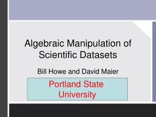
1. Algebraic Manipulation of Scientific Datasets Bill Howe and David Maier OGI School of Science and Engineering at Oregon Health and Science University Portland State University

2. Environmental Observation and Forecastingon the Columbia River Data Products Sensors Simulation

3. Gridded Scientific Datasets 3.2 3.1 3.3 3.2 3.6 3.4 3.6 4.0 3.6 3.8 4.0 4.1 4.0 4.0 4.0 4.0 4.0 12.6C 13.2C 12.5C 13.1C 12.8C 12.1C

4. Some CORIE Grids H = 2d Horizontal Grid T = 1d Time Grid V = 1d Vertical Grid (not shown) Mean Sea Level Underground

5. Thesis • Grid topology requires explicit data model support. • Transformations can be expressed via composition of a few logical operators. • Performance can be preserved via algebraic optimization and specialized operator implementations.

6. Roadmap • Domain Introduction • Model Introduction • Conventional Approaches • Examples of Optimization • Conclusion

7. Grid Topology A collection of cells of various dimensions, implicit or explicit incidence relationships Grid Topology 1 m n q A 0 B p 2 o 3 2-Cells = {A,B} 1-Cells = {m,n,o,p} 0-Cells = {0,1,2,3}

8. Grid Properties • Topology <> geometry • A grid may contain cells of • multiple dimensions • multiple “shapes” • Dimension of a grid is the maximum dimension of its cells 1 n m 2 r A 0 B o q 4 p 3

9. GridField: Grid with Bound Data • Tuples of numeric primitives • Total functions over cells of dimension k • Two gridfields may share a grid

10. Roadmap • Domain Introduction • Model Introduction • Conventional Approaches • Examples of Optimization • Conclusion

11. 1) Modeling with Relations Cell Data • trivial join dependency embedded in the key • decomposition won’t help • no notion of “grid” Node Data G Incidence G

12. 2) Spatial Extensions Node Data • Incidence relationship dependent on geometry rather than topology • Geometry information redundantly defined in nodes and cells • No concept of a “grid”: impedance mismatch with visualization applications Cell Data

13. 3) Visualization Libraries • Different algorithms, each dependent on data characteristics. • Programmer’s responsibility to match algorithms with data • Logical equivalences are obscured Grid restriction: restrict vtkExtractGeometry vtkThreshold vtkExtractGrid vtkExtractVOI vtkThresholdPoints With VTK:

14. Roadmap • Domain Introduction • Model Introduction • Conventional Approaches • Examples of Optimization • Conclusion

15. Operators Task Operator • associate grids with data • combine grids topologically • reduce a grid using data values • transform grids or data • bind (b) • union, intersection, cross product () • restrict (r) • aggregate (a)

16. Restrict Semantics 19 25 21 26 25 25 Values bound to 0-cells (nodes) 19 24 24 restrict(<24) 21 27 27 26 26 24 Values bound to 2-cells (triangles) 25 restrict(<24) 26

17. Working With GridFields “wetgrid” H : (x,y,b)  r(z>b) render r(region) b(s) V : (z) b(r(H  V)) r(b(r(H  V))) (H  V) r(H  V) H V

18. Optimize: Push Restricts G' = G = salt' = salt = s1 s2 s1 s3 s3 s4 s5 s5 temp'= temp = t1 t2 t3 t4 t5 t1 t3 t5 : : : : • salt,temp defined on G • Materialize pointers to elements of salt, temp • Bind salt, temp to a subgrid of G, G' r(p(x,y)) H : (x,y,b) r(z>b) b(s)  r(p(z)) V : (z)

19. Optimization Results

20. Horizontal Slice H(x,y,b)  r(z>b) slice b(s) V(z) r(z>b) b(s) apply H(x,y,b) <depth>

21. Transect (Vertical Slice) H(x,y,b)  r(z>b) “join” b(s) V(z)  P P  V

22. Transect (Vertical Slice) A B H(x,y,b) b(s) “join”  “join” P  V(z) C P

23. A

24. B C

25. Transect Optimizations