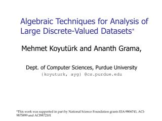
Algebraic Techniques for Analysis of Large Discrete-Valued Datasets 

1. Algebraic Techniques for Analysis of Large Discrete-Valued Datasets Mehmet Koyutürk and Ananth Grama, Dept. of Computer Sciences, Purdue University {koyuturk, ayg} @cs.purdue.edu *This work was supported in part by National Science Foundation grants EIA-9806741, ACI-9875899 and ACI9872101

2. Motivation • Handling large discrete-valued datasets • Extracting relations between data items • Summarizing data in an error-bounded fashion • Clustering of data items • Finding concise interpretable representations for clustered data • Applications • Association rule mining • Classification • Data partitioning & clustering • Data compression

3. Algebraic Model • Sparse matrix representation • Each column corresponds to an item • Each row corresponds to an instance • Document-Term matrix (Information Retrieval) • Columns: Terms • Rows: Documents • Buyer-Item matrix (Data Mining) • Columns: Items • Rows: Transactions • Rows contain patterns of interest!

4. Basic Idea • Not all such matrices are rank 1 (cannot be represented accurately as a single outer product) • We must find the best outer product • Concise • Error-bounded x : presence vector y : pattern vector

5. An Example • Consider the universe of items • {bread, butter, milk, eggs, cereal} • And grocery lists • {butter, milk, cereal} • {milk, cereal} • {eggs, cereal} • {bread, milk, cereal} • These lists can be represented by a matrix as follows:

6. An Example (contd.) • This rank-1 approximation can be interpreted as follows: • Item set {milk, cereal} is characteristic to three buyers • This is the most dominant pattern in the data

7. Rank-1 Approximation • Problem:Given discrete matrixAmxn , find discrete vectorsxmx1andynx1to Minimize ||A-xyT||2F, thenumber of non-zeros in the error matrix • NP-hard! • Assuming continuous space of vectors and using basic algebraic transformations, the above minimization reduces to: Maximize (xTAy)2/ ||x||2||y||2

8. Background • Singular Value Decomposition (SVD) [Berry et.al., 1995] • Decompose matrix into A=USVT • U, V orthogonal, Scontains singular values • Decomposition based on underlying patterns • Latent Semantic Indexing (LSI) • Semi-Discrete Decomposition (SDD) [Kolda & O’Leary, 2000] • Restrict entries of U and V to {-1,0,1} • Can perform as well as SVD in LSI using less than one-tenth the storage[Kolda & O’Leary, 1998]

9. Alternating Iterative Heuristic • In continuous domain, the problem is: minimizeF(d,x,y)=||A-dxyT||F2 F(d,x,y)=||A|| F2-2d xTAy+ d2||x||2||y||2 (1) • Setting F/d = 0gives us the minimum of this function at d*=xTAy/||x||2||y||2 (for positive definite matrix A) • Substituting d* in (1),we get equivalent problem:maximize (xTAy)2/ ||x||2||y||2 • This is the optimization metric used in SDD’s alternating iterative heuristic

10. Approximate binary optimization metric to that of continuous problem Set s=Ay/||y||2, maximize (xTs)2/||x||2 This can be done by sorting s in descending order and assigning 1’s to components of x in a greedy fashion Optimistic, works well on very sparse data Example Alternating Iterative Heuristic 1 1 1 0 1 1 0 0 0 0 1 1 A= y0= [1 0 0 0]  sx0 = Ay = [1 1 0]T  x0= [1 1 0]T  sy0 = ATy = [2 2 0 0]T  y1= [1 1 0 0]  sx1 = Ay = [2 2 0]T  x1= [1 1 0]T

11. Initialization of pattern vector • Crucial to find appropriate local optima • Must be performed in at most (nz(A)) time • Some possible schemes • Center: Initialize y as the centroid of rows, obviously cannot discover a cluster. • Separator: Bipartition rows on a dimension, set center of one group as initial pattern vector. • Greedy graph growing: Bipartition rows with starting from one row and growing a cluster centered on that row in a greedy manner, set center of that cluster as initial pattern vector. • Neighborhood: Randomly select a row, identify set of all rows that share a column with it, set center of this set as initial pattern vector. Aims at discovering smaller clusters, more successful.

12. Recursive Algorithm • At any step, given rank-one approximationAxyT, splitA toA1and A0 based on rows • ifxi=1 rowi goes intoA1 • if xi=0 rowi goes intoA0 • Stop when • Hamming radius ofA1 is less then some threshold • all rows ofAare present inA1 • if Hamming radius of A1greater than threshold, partition based on hamming distances to pattern vector and recurse

13. Example: Recursive Algorithm set =1 1 1 1 0 1 1 1 0 1 0 1 1 A= Rank-1 Appx.: y = [1 1 1 0] x = [1 1 1]T  h.r. = 2 >  A  1 1 1 0 1 1 1 0 1 0 1 1

14. Effectiveness of Analysis Input: 4 uniform patterns intersecting pairwise, 1 pattern on each row(overlapping patterns of this nature are particularly challenging for many related techniques) Detected patterns Input permuted to demonstrate strength of detected patterns

15. Effectiveness of Analysis Input: 10 gaussian patterns, 1 pattern on each row Detected patterns Permuted input

16. Effectiveness of Analysis Input: 20 gaussian patterns, 2 patterns on each row Detected patterns Permuted input

17. Application to Data Mining • Used for preprocessing data to reduce number of transactions for association rule mining • Construct matrix A: • Rows correspond to transactions • Columns correspond to items • Decompose A into XYT • Y is the compressed transaction set • Each transaction is weighted by the number of rows containing the pattern (# of non-zeros in the corresponding row of X)

18. Application to Data Mining (contd.) • Transaction sets generated by IBM Quest data generator • Tested on 10K to 1M transactions containing 20(L), 100(M), and 500(H) patterns • A-priori algorithm ran on • Original transaction set • Compressed transaction set • Results • Speed-up in the order of hundreds • Almost 100% precision and recall rates

19. Preprocessing Results

20. Precision & Recall on M100K

21. Speed-up on M100K

22. runtime vs # columns runtime vs # rows runtime vs # nonzeros Run-time Scalability • Rank-1 approximation requires O(nz(A)) time • Total run-time at each level in the recursive tree can't exceed • this since total # of non-zeros at each level is at most nz(A) • Run-time is O(kXnz(A)) where k is the number of discovered patterns Run-time on data with 2 gaussian patterns on each row

23. Conclusions and Ongoing Work • Scalable to extremely high-dimensions • Takes advantage of sparsity • Clustering based on dominant patterns rather than pairwise distances • Effective in discovering dominant patterns • Hierarchical in nature, allowing multi-resolution analysis • Current work • Parallel implementation

24. References • [Berry et.al., 1995] M. W. Berry, S. T. Dumais, and G. W. O'Brien, Using linear algebra for intelligent information retrieval, SIAM Review, 37(4):573-595, 1995. • [Boley, 1998] D. Boley, Principal direction divisive partitioning (PDDP),Data Mining and Knowledge Discovery, 2(4):325-344, 1998. • [Chu & Funderlic, 2002] M. T. Chu and R.E. Funderlic, The centroid decomposition: relationships between discrete variational decompositions and SVDs, SIAM J. Matrix Anal. Appl., 23(4):1025-1044, 2002. • [Kolda & O’Leary, 1999] T. G. Kolda and D. O’Leary, Latent semantic indexing via a semi-discrete matrix decomposition, In The Mathematics of Information Coding, Extraction and Distribution, G. Cybenko et al., eds., vol. 107 of IMA Volumes in Mathematics and Its Applications. Springer-Verlag, pp. 73-80, 1999. • [Kolda & O’Leary, 2000] T. G. Kolda and D. O’Leary, Computation and uses of the semidiscrete matrix decomposition, ACM Trans. On Math. Software, 26(3):416-437, 2000.