Download

1 / 25
250 likes | 272 Views
Learn the importance of estimating the cost of capital and how to calculate the Weighted Average Cost of Capital (WACC) for making sound financial decisions in corporate finance. Explore methods to determine the cost of equity, debt, and preferred stock to maximize shareholder value.

E N D
Cost of Capital MF 807 Corporate Finance Professor Thomas Chemmanur
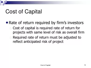
Cost of Capital • Cash flows of a project should be discounted at the opportunity cost of capital, defined as: • the rate of return which can be achieved by the investors in the firm in the best available alternative investment opportunity of the same riskiness of the project • If the project has a positive NPV at this discount rate, the value of the firm’s shares will go up by undertaking the project. • Conversely if the project has a negative NPV, the value of the shares will go down. To maximize shareholder value, managers should not undertake negative NPV projects. • That said, it can be difficult to estimate the cost of capital (as well as to accurately estimate project cash flows) 2
Weighted Average Cost of Capital This method is applicable if: (a) the project being considered is of the same level of riskiness as the existing projects of the firm (b) the capital structure of the firm will remain the same after the project has been financed as it was before it was financed When we study the financing decision, we will see how it is possible to use this method even when (b) is violated. By capital structure, we mean the proportion of firm value represented by the value of each security, e.g. the value of a firm (V), with debt (D), equity (E), and preferred stock (S): 3
Weighted Average Cost of Capital E is the total market value of all common shares outstanding D is the total market value of all bonds issued by the firm S is the total market value of preferred stock issued by the firm Dividing (1) through by V, we obtain: Each term represents a “capital structure” proportion of firm value. Applying these weights to the rate of return required by equity holders, debt holders and preferred stock holders, respectively, gives us the weighted average cost of capital. 4
Weighted Average Cost of Capital Assumptions (a) and (b) are important because, if they hold, we can make use of available data on the market prices of the all the securities issued by the firm in computing the cost of capital to be used in evaluating the project. Assumption (a) means that the riskiness of the securities issued by the firm will not change even after undertaking the project. If the firm undertakes a project of much higher risk than the existing projects of the firm, the systematic risk of the firm’s debt and equity will change, and we can no longer use past information about rates of return. Similarly, if the capital structure changes, again the systematic risk of the firm’s debt and equity will change (we will see how), and we will have to modify the available data in order to use it. 5
Weighted Average Cost of Capital Let us assume that assumptions (a) and (b) do hold. If the firm’s stock beta, denoted by ßE is known, and we know the parameters of the Capital Asset Pricing Model (CAPM), i.e. the risk free rate rF and the expected return on the market rM, we can compute the rate of return demanded by equity holders (“cost of equity”) according to: Another way we can estimate rE is from the constant dividend growth model we studied before. For this, we need to know the growth rate g in dividends expected by investors. Then, if PE is the price per share of the firm’s equity, and D1 is the dividend the firm expects to pay in the next period, the cost of equity is: 6
Weighted Average Cost of Capital The choice of method for computing the cost of equity will depend on how good an estimate we think we have of g versus the CAPM parameters, and on our belief in the validity of the CAPM. Of course, if our estimates are completely accurate, either method should give the same answer. Now, we should compute the cost of debt, rD. This can be computed as the yield to maturity of the bonds issued by the company, which we learned to compute when we studied bond valuations. 7
Weighted Average Cost of Capital We thus know that rD is that this is that value of r which satisfies: Where PD is the current price of each of the firm’s debt (bonds), C is the amount of coupon payments per period, n is the number of periods to maturity and F is the face value of debt. rD is the rate of return expected by bond holders for the firm’s debt. If there is any preferred stock in the firm’s capital structure, we can also compute the cost of preferred equity, which is the rate of return demanded by preferred equity holders, rPE: 8
Weighted Average Cost of Capital The weighted average cost of capital can now be computed as the weighted average of these rates of return rE, rD and rPE, where the weights are the proportions of these securities in the capital structure of the firm. However, we also need to make an adjustment for the fact that interest payments by the company on any bonds issued by the company are deductible from the taxable income of the firm for corporate tax purposes. Let TC represent the marginal corporate tax rate. Making this adjustment to the required return on debt, the formula for the weighted average cost of capital (WACC) is: 9
Weighted Average Cost of Capital Of course, if there is no preferred stock in the firm’s capital structure (as is the case with many firms), the last term in the above formula for the weighted average cost of capital can be omitted. Equation (7) gives the return that investors expect from their investment in the firm’s projects: in other words, it is the required rate of return, or the rate of return to be used in discounting project cash flows. 10
Example Cost of debt, rD = 14% Cost of equity = 500,000 / 7,000,000 + 0.11 = 18.14% Weighted average cost of capital: 11
The Asset Beta Method In many cases, the two assumptions we have made in computing the weighted average cost of capital will not hold. In this case, using an “asset beta” can be helpful. The asset beta of a firm measures the systematic risk of the firm’s assets or projects. In general, it is different from the equity beta, which is the beta of the firm’s stock. To understand what the asset beta measures, it is useful to study the following example. Consider a firm with three different divisions: The first is a division that makes food products The second division makes electronics products The third makes chemicals. 12
The Asset Beta Method Cash flows connected with each division have different levels of systematic risk. The food industry has an average beta of 1 The electronics industry has an average beta of 1.6 The chemicals industry has an average beta of 1.22 Now assume the food division is ½ of the value of the firm, the electronics division is ¼ and the chemical division is ¼. Now assume rF = 5% and rM = 12% The asset beta for the entire firm is given by: 13
The Asset Beta Method The required return on the firm as a whole is: For each division, it is: r1 = 5 + 1(12 – 5) = 12% r2 = 5 + 1.60(12 – 5) = 16.2% r3 = 5 + 1.22(12 – 5) = 13.54% Cross-checking our results by computing the expected return on the entire firm, we have: 14
The Asset Beta Method If all projects in the same division have the same riskiness, then we use a divisional cost of capital to evaluate projects. But it is conceivable that projects within the same division may differ in risk, in which case we should compute individual project betas (which is quite difficult to do). The principle illustrated by the example is that each project should be discounted at the rate of return corresponding to the riskiness of the individual project, as measured by the beta of the individual project. A sample of industry betas: Agriculture, food = 0.99 Media = 1.39 Energy, utilities = 0.60 Banks = 0.81 Air transport = 1.80 Liquor = 0.89 15
Relating Asset and Equity Betas For a firm financed only by debt and equity, V = E + D The beta of a firm must be the weighted average of the betas of the equity and debt betas, where the weights are the respective proportions of equity and debt in the capital structure of the firm. We can simplify and rewrite this as: 16
Relating Asset and Equity Betas The last expression gives us a way of predicting how the equity beta ßEof a firm changes in response to changes in its capital structure. If we assume that the debt beta ßD is constant (which is usually the case; for debt with no default risk, debt beta is zero; even for risky debt, it usually takes very low values except for debt of very high default risk) we can see from the above expression that the riskiness of equity, as measured by the equity beta of the firm, increases as the debt-equity ratio goes up. Let ßD = 0. With E/V = ½ and D/V = ½, we have: 17
Relating Asset and Equity Betas Remember that, irrespective of how the firm is financed, the asset beta of the firm is always a constant for a given set of projects undertaken by the firm, since the asset beta reflects only on the business risk of the firm. The asset beta of a firm changes only if the firm changes its portfolio of projects, i.e. only if the firm undertakes additional projects with a systematic risk different from those of the existing projects of the firm. The equity beta thus reflects the financial risk as well as the business risk of the firm The asset beta reflects only the business risk of the firm. The asset beta will equal the equity beta only for the special case where the firm is 100% equity financed. (E/V = 1, D/V = 0) 18
Relating Asset and Equity Betas Further, it is clear that if the firm is 100% equity financed, the equity of the firm will have only the business risk of the firm, while introducing debt into the capital structure also subjects the equity holders to financial risk. How can we use the concepts we have learned above to compute the cost of capital of a project which has a riskiness different from those of existing projects in the firm, and which will also lead to changes in the firm’s capital structure? The following steps are involved: 1. Compute the beta of the project, either from the beta of the industry in which the project is undertaken, or from computing the asset beta of a firm similar to ours in the same industry as the project, assuming that the beta of the project we are evaluating is the same. 19
Relating Asset and Equity Betas 2. Using the CAPM, compute the expected return corresponding to this project beta. Call this rate of return rA. 3. Adjust the rate of return we got in step (2) for the tax deductibility of payments to debt holders, using the “target” proportion of debt to be used in financing the project, denoted by L. Thus, if TC is the corporate tax rate, then the cost of capital r to be used to discount the project’s cash flows is given by (10): Notice that in (10), L can be higher or lower than the proportion of debt in the current capital structure of the firm, D/V. 20
Relating Asset and Equity Betas Further, L may also differ in some cases from the proportion of debt used to meet the immediate financing needs of the project. L should reflect the proportion of the project’s investment requirement that is to be financed by debt in the long run target capital structure. We make the adjustment in (10) to incorporate the fact that interest payments on debt are deductible for corporate tax purposes. Caution: the tax adjustment formula is an approximation, and will hold exactly only under certain restrictive assumptions about personal tax rates of investors and the nature of the debt used to finance the project. This topic is somewhat controversial, and you will find different formulae in different textbooks, though all of them will compute reasonably close figures for the cost of capital. 21
Example (a) ßD = 0 for Rivolta , ßA = (E/V) ßE = 0.8 (2) = 1.6 (b) Asset beta of your firm = 1.6, same as Rivolta rA = 10 + 1.6 (19 – 10) = 24.44% r = 24.4 (1 – 0.4 ) = 20.496% (c) 1.6 = ßA = 0.6 ßE + 0.4(0.1) = 0.6 ßE + 0.04 (since ßD = 0.1) ßE = (1.6 – 0.04) / 0.6 = 2.6 Note if ßD = 0, ßE = 1.6 / 0.6 = 2.66 22
Concluding Comments We have discussed above two different methods of finding the cost of capital in evaluating projects. The weighted average cost of capital method can be used when we know that the project being undertaken is of the same riskiness as the existing projects in the firm, and the capital structure of the firm will remain unchanged even after the project is undertaken. The asset beta can be used when we know that these assumptions do not hold. If the above two assumptions hold, either method will give approximately the same answer. “Approximately”, because the adjustment for the tax deductibility of corporate payments to debtholders works only approximately in various settings. 23
Concluding Comments Throughout our discussion, we have assumed that only systematic or “market” risk matters in evaluating projects. However, in practice, many corporate managers also worry about idiosyncratic (i.e. firm-specific) risk, perhaps because of concerns for bankruptcy costs and their own career concerns or perhaps because they believe that, in reality, investors in the economy do not hold well diversified portfolios and therefore that the CAPM is not the correct model to use. These kinds of concerns make the estimation of the cost of capital still something of an art, however the techniques we have studied above can at least provide valuable starting figures for further analysis. 24
Concluding Comments In summary, we learned in the last several classes how firm managers should make the investment decision: 1. They should estimate the cash flow stream associated with each project, and compute the expected cash flow at each point in time 2. They should then find the NPV of the project, discounting project cash flows at a cost of capital corresponding to the riskiness of the project cash flow stream. 3. The optimal investment decision rule is then to accept all positive NPV projects if there is no capital rationing; if there is rationing, they should choose that set of projects which, while satisfying any investment constraint, gives the largest NPV. Such a decision maximizes firm value. 25