Download

1 / 48
480 likes | 492 Views
Explore terms, hypotheses testing, power, and sample size in statistical analysis using PASS software. Learn hypothesis logic, types, and research design with examples and software manuals. Understand the USA legal system's statistical viewpoint on innocence and guilt. Discover the concept of statistical power and its significance in decision-making. Dive into error types, confidence levels, and distribution analyses. Gain insights into sample size determination with practical examples and references to statistical studies.

E N D
A Practical Approach to Power, Effect Size and Sample Size&Introduction to PASS(Power Analysis and Sample Size software) Melinda K. Higgins, Ph.D. 30 January 2013
Outline • Terms and Definitions • Logic & Pictures • Hypotheses About One Mean (Example and Intro to PASS) • Types of Hypotheses • PASS Overview – software introduction and manuals • Examples: • Summary & Statistical Power Software List (links & $) • Contact Info
Hypothesis Testing • USA Legal System: “We ASSUME that a person is INNOCENT until PROVEN GUILTY.” • Null Hypothesis (“Status Quo”) • H0: Person = Innocent • Alternative Hypothesis (“What We’d Like to PROVE”) • Ha: Person = Guilty • “Burden of Proof” is on Prosecution [There has to be ENOUGH EVIDENCE to REJECT Innocence and CONCLUDE GUILT.] • Underlying Structure – we’d rather let a guilty person go free than send an innocent person to jail… more later…
From a Stats Point of View • Null Hypothesis [H0]: The Hypothesis to be “Tested” – really this is what we want to reject in favor of the Alternative Hypothesis • Alternative Hypothesis [Ha]: The stated alternative to the null – really what we would like to “accept” and “conclude” • Hypothesis Test: The test performed to make the decision to either “Accept Ha” or “Not Reject H0” • ** NEVER ACCEPT THE NULL HYPOTHESIS ** Always State that “there was not enough evidence to reject the null hypothesis – this does NOT mean the Null Hypothesis is True. [Just because the prosecution could not prove their case does not mean the defendant is innocent.]
POWER – Some initial terms and definitions • H0 is the Null Hypothesis (want to reject this to conclude Ha – the alternative hypothesis) • Ha is the Alternative Hypothesis (ideally this is the conclusion you want to reach) • If statistical significance is found (p-value < ), “You reject the null and accept the alternative hypothesis.” • If the test is NOT significant you state that “You can not reject the null hypothesis.” • YOU NEVER ACCEPT THE NULL HYPOTHESIS!! ** Research Design ** US Legal System
Types of “Error” “Truth” “Ha is True (H0 is false)” “H0 is True” 1- Confidence Level Type II error Fail to Reject H0 “Result” POWER 1- Type 1 error Reject H0, Conclude Ha • Type I Error (Significance Level): Rejecting the Null Hypothesis when it is in fact true • Type II Error (): Not Rejecting the Null Hypothesis when it is in fact false.
Type II error 1- POWER Type 1 error Power – The pictures DISTRIBUTION UNDER ALTERNATIVE HYPOTHESIS DISTRIBUTION UNDER NULL HYPOTHESIS H0 : μ0=μa Ha : μ0<μa Type II error 1- POWER Type 1 error Notice that everything depends on the “critical value” = 108.2, which depends on alpha ()
What if μ0=100, μa=105 (σx=20 & N=16) ?Closer together – will power increase or decrease? Power = 0.26 (previously was 0.64) μa-μ0=5 (previous difference = 10)
What if μ0=100, μa=115 (σx=20 & N=16) ? Power = 0.91 (was 0.64) μa-μ0=15 (previous difference = 10)
Power = 0.64 What if μ0=100, μa=105 (σx=10, N=16) ?What if μ0=100, μa=110 (σx=10, N=16) ?What if μ0=100, μa=115 (σx=10, N=16) ? Power = 0.99 Power = 1.00 If we decrease x, will power go up or down? The “effect” of increasing the difference between the means increases power, i.e. μa-μ0 is related to “effect size” of this test.
Summary so far This is for N=16, what if we have a different N (sample size)?
Link to BIOS 500 Power Homework • BIOS 500 Power Homework
PASS Results – 1 Mean (page 1) Numeric Results for One-Sample T-Test Null Hypothesis: Mean0=Mean1 Alternative Hypothesis: Mean0<Mean1 Known standard deviation. Effect Power N Alpha Beta Mean0 Mean1 S Size 0.63876 16 0.05000 0.36124 100.0 105.0 10.0 0.500 0.25951 16 0.05000 0.74049 100.0 105.0 20.0 0.250 0.99074 16 0.05000 0.00926 100.0 110.0 10.0 1.000 0.63876 16 0.05000 0.36124 100.0 110.0 20.0 0.500 0.99999 16 0.05000 0.00001 100.0 115.0 10.0 1.500 0.91231 16 0.05000 0.08769 100.0 115.0 20.0 0.750 References Machin, D., Campbell, M., Fayers, P., and Pinol, A. 1997. Sample Size Tables for Clinical Studies, 2nd Edition. Blackwell Science. Malden, MA. Zar, Jerrold H. 1984. Biostatistical Analysis (Second Edition). Prentice-Hall. Englewood Cliffs, New Jersey. Notice – Effect Size depends on BOTH the difference between μ0 and μa and the standard deviation
PASS Results – 1 Mean (page 2) Report Definitions Power is the probability of rejecting a false null hypothesis. It should be close to one. N is the size of the sample drawn from the population. To conserve resources, it should be small. Alpha is the probability of rejecting a true null hypothesis. It should be small. Beta is the probability of accepting a false null hypothesis. It should be small. Mean0 is the value of the population mean under the null hypothesis. It is arbitrary. Mean1 is the value of the population mean under the alternative hypothesis. It is relative to Mean0. Sigma is the standard deviation of the population. It measures the variability in the population. Effect Size, |Mean0-Mean1|/Sigma, is the relative magnitude of the effect under the alternative. Summary Statements A sample size of 16 achieves 64% power to detect a difference of 5.0 between the null hypothesis mean of 100.0 and the alternative hypothesis mean of 105.0 with a known standard deviation of 10.0 and with a significance level (alpha) of 0.05000 using a one-sided one-sample t-test. ** Can Cut and Paste This into Proposals!! **
PASS Results – 1 Mean (page 3) Power increases as “effect size” increases.Power increases as standard deviation decreases.
PASS Results – What about for N=25?Will Power go up or down? Power increases as sample size increases.
Sample Size to Achieve Power Vs Power = 80% when N=25, for Mean0=100, Stdev=10 for Mean1=105 Power = 80% when N=25, for Mean0=100, Stdev=20 for Mean1=110
Effect Size and the Alternative Hypothesis: ** Subtle but Key Concepts ** • Typically the alternative hypothesis (Ha) gives the direction of the difference from the null hypothesis (H0) but not how different. • H0: 0=a versus Ha: 0≠a; 0<a; or 0>a • Thus, the power is calculated at specific alternative values. These values should be considered as values at which the power is calculated and NOT AS THE TRUE value. • Effect size is the change in the parameter of interest that is to be detected (NOT the actual change seen). • Clinical significance Vs. Statistical significance • (e.g. is a difference of 3 yrs in age important? 2 lbs of weight loss? – adult vs. baby)
Types of Hypotheses ** Terminology Used in PASS ** • Inequality Hypothesis (two values unequal) • Two-sided Inequality • One-sided Inequality (no preference specified) • One-sided Non-inferiority (one not worse than another) • One-sided Superiority (one better than another by specified amount) • Equivalence (no difference within specified margin) Most Common
Types of Power Analyses: • Pre-study • Determine the sample size (N) based on alpha and beta (and effect size of interest) • Post-study (post hoc questions) • What sample size would have been needed to detect a specific effect size? (effect size of interest – not what was seen) • What is the smallest effect size that could be detected with this sample size? (the size at the end of the study) • What was the power of the test procedure(s)? [Note: Multiple statistical tests can be employed]
PASS Intro and Examples • PASS Layout • PASS Manuals [1432 pages total] • User’s Guide – I “Quick Start, Proportions, and ROC Curves” • User’s Guide – II “One Mean, Two Means, and Cross-Over Designs” • User’s Guide – III “ANOVA, Multiple Comparisons, Simulator, Variances, Survival Analysis, Correlations, Regression, and Helps” • PASS Examples: • Section 250 – Many Proportions: Chi-Square Test • Section 400 – One Mean: Inequality (Normal) PREVIOUS EXAMPLE • Section 400 – Example 4 – Difference of Two-Paired Means • Section 430 – Two Independent Means: Inequality (Normal) • Section 800 – Correlations: One (Pearson) Correlation • Section 810 – Correlations: Intraclass Correlation (ICC)
Everyone should read Will be addressed within other statistical lectures Similar to Means (400-495) Quality Measures Estimation of “Nuisance Parameters”
Effect Size (for t-test)[Cohen, J. “Statistical Power Analysis for the Behavioral Sciences (2nd ed)” (1988)] • Example for t-test: • Cohen’s d • d = 0.2 “small” • meaning that the difference in the means is 20% as large as the “common” standard deviation. So, if the standard deviation in a particular measure is +/- 10, a small effect size would be a difference of 2. • d = 0.5 “medium” • d = 0.8 “large” • Use these numbers as guidelines for your study. Calculate an approximate ratio of the expected difference in means divided by a conservative (largest) estimate for the standard deviation.
Numeric Results for Two-Sample T-Test Null Hypothesis: Mean1=Mean2. Alternative Hypothesis: Mean1<>Mean2 The standard deviations were assumed to be unknown and equal. Allocation Power N1 N2 Ratio Alpha Beta Mean1 Mean2 S1 S2 0.80003 1570 1570 1.000 0.05000 0.19997 0.000 0.100 1.000 1.000 0.80044 393 393 1.000 0.05000 0.19956 0.000 0.200 1.000 1.000 0.80138 176 176 1.000 0.05000 0.19862 0.000 0.300 1.000 1.000 0.80365 100 100 1.000 0.05000 0.19635 0.000 0.400 1.000 1.000 0.80146 64 64 1.000 0.05000 0.19854 0.000 0.500 1.000 1.000 0.80370 45 45 1.000 0.05000 0.19630 0.000 0.600 1.000 1.000 0.81165 34 34 1.000 0.05000 0.18835 0.000 0.700 1.000 1.000 0.80749 26 26 1.000 0.05000 0.19251 0.000 0.800 1.000 1.000 0.81211 21 21 1.000 0.05000 0.18789 0.000 0.900 1.000 1.000 0.80704 17 17 1.000 0.05000 0.19296 0.000 1.000 1.000 1.000 Since the standard deviation of each group = 1, and Mean1 (for the 1st group) is set = to 0, then Mean2 is the effect size of interest. This table presents results for effect sizes from 0.1 to 1.0. Thus, you need 393 per group (786 total) to “detect” an effect size of 0.2
Remember that N1=N2, so the sample sizes represented here have to be doubled to estimate total sample sizes needed. So, for a sample size of 100+100 (200 total), we can “detect” an effect size of 0.4 (M2).
Section 430 – Two Independent Means: Inequality (Normal) Setup: A clinical trial was run to compare the effectiveness of two drugs (results below). Calculate power for various sample sizes and alpha = 0.01 and 0.05 (given each group’s sample mean and stddev).
Parameters Find = Beta Mean1 = 20.9 Mean2 = 17.8 N1 = 5 to 50 by 5 N2 = Use R R = 1 [N1=N2] Alt Hyp = Ha: Mean1 <> Mean2 Parameters (cont’d) Nonparametric Adjustment (ignore) Alpha = .01 .05 Beta (ignored since this is find setting) S1 = 3.67 [“Helps” Button] S2 = 3.01 Known SD (unchecked) [Axes TAB] Vertical Range: Set Min=0, Max=Data Two Independent Means
Summary Statements Group sample sizes of 20 and 20 achieve 81% power to detect a difference of 3.1 between the null hypothesis that both group means are 20.9 and the alternative hypothesis that the mean of group 2 is 17.8 with estimated group standard deviations of 3.7 and 3.0 and with a significance level (alpha) of 0.05000 using a two-sided two-sample t-test.
Parameters Find = N Mean0 = 0 Mean1 = 5 N (this is the find setting) StdDev = 10 12.5 15 (unknown) Parameters (cont’d) Population size = infinite Alt Hypothesis = Ha: Mean0 <> Mean 1 Nonparametric adjustment (ignore) Alpha = 0.01 0.05 Beta = 0.20 Section 400 – Example 4 – Difference of Two-Paired Means: Inequality Setup: Weight Loss – Pre vs. Post Exercise Program – Past experiments of this type have had standard deviations of 10-15 lbs. The researcher wants to detect a difference of 5 lbs or more (either way). Alpha values of 0.01 and 0.05 will both be evaluated. Beta is set to 0.20 (for 80% power). What sample size is needed?
Numeric Results for One-Sample T-Test Null Hypothesis: Mean0=Mean1 Alternative Hypothesis: Mean0<>Mean1 Unknown standard deviation. Effect Power N Alpha Beta Mean0 Mean1 S Size 0.80939 51 0.01000 0.19061 0.0 5.0 10.0 0.500 0.80778 34 0.05000 0.19222 0.0 5.0 10.0 0.500 0.80434 77 0.01000 0.19566 0.0 5.0 12.5 0.400 0.80779 52 0.05000 0.19221 0.0 5.0 12.5 0.400 0.80252 109 0.01000 0.19748 0.0 5.0 15.0 0.333 0.80230 73 0.05000 0.19770 0.0 5.0 15.0 0.333 Summary Statements A sample size of 34 achieves 81% power to detect a difference of -5.0 between the null hypothesis mean of 0.0 and the alternative hypothesis mean of 5.0 with an estimated standard deviation of 10.0 and with a significance level (alpha) of 0.05000 using a two-sided one-sample t-test.
Numeric Results for One-Sample T-Test – for generic approach Null Hypothesis: Mean0=Mean1 Alternative Hypothesis: Mean0<>Mean1 Unknown standard deviation. Effect Power N Alpha Beta Mean0 Mean1 S Size 0.80169 199 0.05000 0.19831 0.000 0.200 1.000 0.200 “small” 0.80379 90 0.05000 0.19621 0.000 0.300 1.000 0.300 0.80779 52 0.05000 0.19221 0.000 0.400 1.000 0.400 0.80778 34 0.05000 0.19222 0.000 0.500 1.000 0.500 “medium” 0.80367 24 0.05000 0.19633 0.000 0.600 1.000 0.600 0.82255 19 0.05000 0.17745 0.000 0.700 1.000 0.700 0.82131 15 0.05000 0.17869 0.000 0.800 1.000 0.800 “large”
Effect Size for Chi-Square • Effect Size for Chi-Square test • Cohen’s “w” • w = 0.1 “small” • indicating that expected Chi-square will be 1% (0.01) of the total sample size (N); w2 = (0.1)2 = 0.01 • w = 0.3 “medium” • w = 0.5 “large” • Use these numbers as guidelines for your study. Typically estimate a Chi-square from previous studies or pilot data.
Section 250 – Chi-Square Tests(Two-way contingency tables) • Two possible tests • Chi-square “goodness of fit” test • Chi-square “test for independence” [*most common*] • Parameters • DF – degrees of freedom = (r-1)(c-1) • W (effect size) • N (sample size) • Alpha (significance level) • Beta (1 – Power)
.01 .05 .10 0.366213 Beta and Power 2 .2 25 to 300 by 25
Summary Statement A sample size of 75 achieves 81% power to detect an effect size (W) of 0.3662 using a 2 degrees of freedom Chi-Square Test with a significance level (alpha) of 0.05000.
Numeric Results for Chi-Square Test – For a 2x2 Table • Power N W Chi-Square DF Alpha Beta • 0.80006 785 0.1000 7.8500 1 0.05000 0.19994 • 0.80155 197 0.2000 7.8800 1 0.05000 0.19845 • 0.80353 88 0.3000 7.9200 1 0.05000 0.19647 • 0.80743 50 0.4000 8.0000 1 0.05000 0.19257 • 0.80743 32 0.5000 8.0000 1 0.05000 0.19257 • NOTE: For a 2x2 table DF=(r-1)(c-1)=(2-1)(2-1)=1 • References: Cohen, Jacob. 1988. Statistical Power Analysis for the Behavioral Sciences, Lawrence Erlbaum Associates, Hillsdale, New Jersey. • Report Definitions • Power is the probability of rejecting a false null hypothesis. It should be close to one. • N is the size of the sample drawn from the population. To conserve resources, it should be small. • W is the effect size--a measure of the magnitude of the Chi-Square that is to be detected. • DF is the degrees of freedom of the Chi-Square distribution. • Alpha is the probability of rejecting a true null hypothesis. • Beta is the probability of accepting a false null hypothesis. • Summary Statements • A sample size of 197 achieves 80% power to detect an effect size (W) of 0.2000 using a 1 degree of freedom Chi-Square Test with a significance level (alpha) of 0.05000.
So, for 2x2 tables (DF=1), you’ll need 197 total to “detect” a small effect size (w) for a Chi-square test; and only 32 for a large effect size.
Effect Size (for Correlation/Regression)[Cohen, J. “Statistical Power Analysis for the Behavioral Sciences (2nd ed)” (1988)] • Correlation (r and r2) IS an Effect Size • “r” • r = 0.1 “small” r2=0.01 • r = 0.3 “medium” r2=0.09 • r = 0.5 “large” r2=0.25 • Use these numbers as guidelines for your study.
Section 800 – Correlations: One (Pearson) Correlation • Setup: Baseline correlation among dyads (Patient-Family Caregiver) by item within an instrument ranged from 0.1 to 0.8. A follow-on trial is planned to test a “treatment” to improve (increase) correlation (congruency) among the dyads (ideally improving correlation for the worst items). • Given a sample size of approximately 40 dyads (reasonable to expect from past recruitment experience), what is the statistical power? And what effect sizes (change in correlation) can be detected? • How large a sample size is required at 80% power to detect smaller improvements in correlation (0.1-0.2).
One (Pearson) Correlation • Parameters • Find = Beta and Power • R0 = 0.1 [lowest seen in baseline (control) group] • R1 = 0.2 to 0.9 by 0.1 (potential improvements) • N = 20 to 200 by 20 • Alt Hyp: Ha: R0 <> R1 • Alpha = 0.05 • Beta (ignored, this is the find setting)
Summary Statements A sample size of 40 achieves 78.9% power to detect a difference of -0.40000 between the null hypothesis correlation of 0.10000 and the alternative hypothesis correlation of 0.50000 using a two-sided hypothesis test with a significance level of 0.05000. A sample size of 180 achieves 79.6% power to detect a difference of -0.2 (R0=0.1, R1=0.3).
Numeric Results – Multivariate Regression; 5 Covariates (R2=0.01) with 2 Predictors (with various adjusted R2; R2 change) [R2=0.02 “small”; R2=0.13 “medium”; R2=0.26 “large”] Ind. Variables Ind. Variables Tested Controlled Power N Alpha Beta Cnt R2 Cnt R2 0.80061 471 0.05000 0.19939 2 0.02000 “small” 5 0.01000 0.80068 130 0.05000 0.19932 2 0.07000 5 0.01000 0.80500 74 0.05000 0.19500 2 0.12000 “med” 5 0.01000 0.80039 50 0.05000 0.19961 2 0.17000 5 0.01000 0.80744 38 0.05000 0.19256 2 0.22000 5 0.01000 0.80648 30 0.05000 0.19352 2 0.27000 “large” 5 0.01000 0.81356 25 0.05000 0.18644 2 0.32000 5 0.01000 0.80955 21 0.05000 0.19045 2 0.37000 5 0.01000 0.80177 18 0.05000 0.19823 2 0.42000 5 0.01000 Summary Statements A sample size of 471 achieves 80% power to detect an R-Squared of 0.02000 attributed to 2 independent variable(s) using an F-Test with a significance level (alpha) of 0.05000. The variables tested are adjusted for an additional 5 independent variable(s) with an R-Squared of 0.01000.
Summary/Points to Remembers • Never accept the null hypothesis. Always state, “We can not reject the null hypothesis.” • Always design your “experiment” to reject the null hypothesis in order to accept the alternative (i.e. what you want to prove), given statistical significance is achieved. • Identify the statistical test(s) appropriate for testing your hypothesis(es). • Use the most conservative (largest) sample size estimate given your “effect size” of interest (i.e. clinically significant not statistically significant).
PASS and Other Power Software • PASS – go to http://www.ncss.com/pass.html [PASS ver 12 single academic license = $795.95 (upgrade from PASS 2011 is $349.00); 7-day FREE trial] [Windows OS required – a Windows emulator (such as Parallels) is required to run PASS 12 on a Mac.] • Power and Precision (BioStat) – go to http://www.power-analysis.com/ [academic perpetual license $595, also has free trial] • StudySize 2.0 – go to http://www.studysize.com/ [14-day FREE trial; $129 for StudySize 2.0] • G*Power 3 – go to http://www.psycho.uni-duesseldorf.de/abteilungen/aap/gpower3/ [FREE] • “Russ Lenth's power and sample-size page” – go to http://www.math.uiowa.edu/~rlenth/Power/ [access JAVA applets online or download for FREE] • For a large list of available “Power, Sample Size and Experimental Design Calculations” – go to http://statpages.org/#Power
Contact Dr. Melinda Higgins Melinda.higgins@emory.edu Office: 404-727-5180 / Mobile: 404-434-1785 VIII. Statistical Resources and Contact Info