Download

1 / 60
600 likes | 771 Views
This chapter covers the operations supported by priority queues, including inserting, deleting, and combining elements based on priority. It discusses single-ended priority queues (SPQ) and double-ended priority queues (DEPQ), detailing methods for returning elements of minimum and maximum priority. Extended binary trees and leftist trees are defined, explaining how leftist trees balance their structure for efficient operations. The chapter also emphasizes the efficiency of combining two priority queues using leftist trees, with clear definitions and mathematical recurrences for shortest paths.

E N D
Chap 9 Priority Queues
Operations supported by priority queue • The functions that have been supported: • SP1: Return an element with minmum priority • SP2: Insert an element with an arbitrary priority • SP2: Delete an element with minimum priority • Extended functions: • Meld two priority queues • delete an arbitrary element • decrease the key/priority
Double-ended priority queue(DEPQ) • Support the following operations • DP1: Return an element with minimum priority • DP2: Return an element with maximum priority • DP3: Insert an element with an arbitrary • DP4: Delete an element with minimum priority • DP5: Delete an element with maximum priority
To combine two priority queues into a single priority queue, the combine operation takes O(n) time if heaps are used. The complexity of combine operation can be reduced to O(log n) if a leftist tree is used. Leftist trees are defined using the concept of an extended binary tree. An extended binary tree is a binary tree in which all empty binary subtrees have been replaced by a square node. The square nodes in an extended binary tree are called external nodes. The original nodes of the binary tree are called internal nodes. Leftist Trees
Extended Binary Trees G A H I B C J D E F
Leftist Trees (Cont.) • Let x be a node in an extended binary tree. Let LeftChild(x) and RightChild(x), respectively, denote the left and right children of the internal node x. • Define shortest(x) to be the length of a shortest path from x to an external node. It is easy to see that shortest(x) satisfies the following recurrence: shortest(x) = 0 if x is an external node 1 + min{shortest(LeftChild(x)), RightChild(x))} otherwise
Shortest(x) of Extended Binary Trees 2 2 G A 1 1 1 2 H I B C 1 1 1 1 J D E F
Definition: A leftist tree is a binary tree such that if it is not empty, then shortest(LeftChild(x)) ≥ shortest(RightChild(x)) for every internal node x. Lemma 9.1: Let x be the root of a leftist tree that has n (internal) nodes n ≥ 2shortest(x) – 1 The rightmost root to external node path is the shortest root to external node path. Its length is shortest(x). Leftist Tree Definition
template<class KeyType>class MinLeftistTree; // forward declaration template<class KeyType> class LeftistNode { friend class MinLeftistTree<KeyType>; private: Element<KeyType>data; LeftistNode *LeftChild, *RightChild; int shortest; } template<class KeyType> class MinLeftistTree:public MinPQ<KeyType> { public: // constructor MinLeftistTree(LeftistNode<KeyType> *int = 0) root(int) {}; // the three min-leftist tree operations void Insert(const Element<KeyType>&); Element<KeyType>* DeleteMin(Element<KeyType>&); void MinCombine(MinLeftistTree<KeyType>*); private: LeftistNode<KeyType>* MinUnion(LeftistNode<KeyType>*, LeftistNode<KeyType>*); LeftistNode<KeyType>* root; }; Class Definition of A Leftist Tree
Definition: A min leftist tree (max leftist tree) is a leftist tree in which the key value in each node is no larger (smaller) than the key values in its children (if any). In other words, a min (max) leftist tree is a leftist tree that is also a min (max) tree. Definition of A Min (Max) Leftist Tree
Examples of Min Leftist Trees 2 2 2 2 1 1 1 1 9 8 50 7 2 1 1 1 12 10 80 11 1 1 1 1 20 18 15 13
Like any other tree structures, the popular operations on the min (max) leftist trees are insert, delete, and combine. The insert and delete-min operations can both be done by using the combine operation. e.g., to insert an element x into a min leftist tree, we first create a min leftist tree that contains the single element x. Then we combine the two min leftist trees. To delete the min element from a nonempty min leftist tree, we combine the min leftist trees root->LeftChild and root->RightChild and delete the node root. Min (Max) Leftist Tree (Cont.)
To combine two leftist trees: First, a new binary tree containing all elements in both trees is obtained by following the rightmost paths in one or both trees. Next, the left and right subtrees of nodes are interchanged as necessary to convert this binary tree into a leftist tree. The complexity of combining two leftist trees is O(logn) Combine Leftist Trees
Combining The Min Leftist Tree 2 2 2 8 1 2 1 1 5 10 50 7 2 1 2 1 1 1 15 8 80 2 11 9 2 2 1 1 1 2 12 13 10 50 7 5 2 1 1 1 5 20 15 18 2 80 1 1 2 8 1 9 11 8 9 1 1 1 2 2 1 1 10 50 12 13 12 10 50 1 1 1 1 15 1 20 80 18 1 20 15 18 80
A binomial heap is a data structure that supports the same functions as those supported by leftist trees. Unlike leftist trees, where an individual operation can be performed in O(log n) time, it is possible that certain individual operations performed on a binomial heap may take O(n) time. By amortizing part of the cost of expensive operations over the inexpensive ones, then the amortized complexity of an individual operation is either O(1) or O(log n) depending on the type of operations. Binomial Heaps
Given a sequence of operations I1, I2, D1, I3, I4, I5, I6, D2, I7. Assume each insert operation costs one time unit and D1 and D2 operations take 8 and 10 time units, respectively. The total cost to perform the sequence of operations is 25. If we charge some actual cost of an operation to other operations, this is called cost amortization. In this example, the amortized cost of I1 – I6 each has 2 time units, I7 has one, and D1 and D2 each has 6. Now suppose we can prove that no matter what sequence of insert and delete-min operations is performed, we can charge costs in such a way that the amortized cost of each insertion is no more than 2 and that of each deletion is no more than 6. We can claim that the sequence of insert/delete-min operations has cost no more than 2*i + 6*d. With the actual cost, we conclude that the sequence cost is no more than i+10*d. Combining the above two bounds, we obtain min{2*i+6*d, i+10*d}. Cost Amortization
Binomial heaps have min binomial heap and max binomial heap. We refer to the min binomial heap as B-heap. B-heap can perform an insert and a combine operation in O(1) actual and amortized time and a delete-min operation with O(log n) amortized time. A node in a B-heap has the following data members: degree: is the number of children it has child: is a pointer points to any one of its children. All children forms a circular list. link: is a singly link used to maintain a circular list with its siblings. data The roots of the min trees that comprise a B-heap are linked to form a singly linked circular list. The B-heap is then pointed at by a single pointer min to the min tree root with smallest key. Binomial Heaps
B-Heap Example 1 3 8 16 12 7 4 10 5 9 30 15 6 min 20 8 1 3 16 10 12 7 4 5 9 30 15 6 20
An element x can be inserted into a B-heap by first putting x into a new node and then inserting this node into the circular list pointed at by min. The operation is done in O(1) Time. To combine two nonempty B-heaps, combine the top circular lists of each into a single circular list. The new combined B-heap pointer is the min pointer of one of the two trees, depending on which has the smaller key. Again the combine operation can be done in O(1) time. Insertion Into A B-Heap
The Tree Structure After Deletion of Min From B-Heap 16 7 12 8 3 10 9 30 15 4 5 20 6
If min is 0, then the B-heap is empty. No delete operations can be performed. If min is not 0, the node is pointed by min. Delete-min operation deletes this node from the circular list. The new B-heap consists of the remaining min trees and the submin trees of the delete root. To form the new B-heap, min trees with the same degrees are joined in pairs. The min tree whose root has the larger key becomes the subtree of the other min tree. Deletion of Min Element
Joining Two Degree-One Min Trees 16 12 3 7 30 8 9 15 4 5 10 20 6
Joining Two Degree-Two Min Trees 3 16 12 7 4 5 30 15 6 8 9 20 10 Since no two min trees have the same degree, the min join process stops.
The New B-Heap min 3 16 12 7 4 5 30 15 6 8 9 20 10
template<class KeyType> Element<KeyType>*Binomial<KeyType>::DeleteMin(Element<KeyType>&x) Step 1: [Handle empty B-heap] if (!min){ DeletionError(); return();} Step 2: [Deletion from nonempty B-heap] x=min->data; y=min->child; delete min from its circular list; following this deletion, min points to any remaining node in the resulting list; if there is no such node, then min = 0; Step 3: [Min-tree joining] Consider the min trees in the lists min and y; join together pairs of min trees of the same degree until all remaining min trees have different degrees; Step 4: [Form min tree root list] Link the roots of the remaining min trees (if any) together to form a circular list; set min to point to the root (if any) with minimum key; return &x; Program 9.12 Steps In A Delete-Min Operation
Binomial Tree Definition • Definition: The binomial tree Bk, of degree k is a tree such that if k = 0, then the tree has exactly one node, and if k > 0, then the tree consists of a root whose degree is k and whose subtrees are B0, B1, …, Bk-1. • Lemma 9.2: Let a be a B-heap with n elements that results from a sequence of insert, combine, and delete-min operations performed on a collection of initially empty B-heaps. Each min tree in a has degree ≤ log2n. Consequently, MaxDegree ≤ , and the actual cost of a delete-min operation is O(log n + s).
Theorem 9.1: If a sequence of n insert, combine, and delete-min operations is performed on initially empty B-heaps, then we can amortize costs such that the amortized time complexity of each insert and combine is O(1), and that of each delete-min operation is O(log n). B-Heap Costs
A Fibonacci heap is a data structure that supports the three binomial heap operations: insert, delete-min (or delete-max), and combine, as well as the following additional operations: decrease key: Decrease the key of a specified node by a given positive amount delete: Delete the element in a specified node. The first of these can be done in O(1) amortized time and the second in O(log n) amortized time. The binomial heap operations can be performed in the same asymptotic times using a Fibonacci heap as they can be using a binomial heap. Fibonacci Heaps
Two varieties of Fibonacci heaps: Min Fibonacci heap: is a collection of min trees Max Fibonacci heap: is a collection of max trees. Refers to min Fibonacci heap as F-heaps. B-heaps are a special case of F-heaps. A node in F-heap data structure contains additional data members other than those in B-heaps: parent: is used to point to the node’s parent (if any). ChildCut: to support cascading cut described later. LeftLink and RightLink: replace the link data member in B-heap node. These links form a doubly linked circular list. In F-heaps, singly linked circular list is replaced by doubly linked circular list. Fibonacci Heaps (Cont.)
The basic operations insert, delete-min, and combine are performed exactly as for the case of B-heaps. Follow the below steps to delete a node b from an F-heap: If min = b, then do a delete-min; otherwise do Steps 2, 3, and 4 below Delete b from its doubly linked list Combine the doubly linked list of b’s children with the doubly linked list pointed at by min into a single doubly linked list. Trees of equal degree are not joined as in a delete-min operation. Dispose of node b. Deletion From An F-Heap
F-Heap After Deletion of 12 8 30 1 3 11 10 20 16 4 7 5 9 6 min 8 30 1 3 11 10 20 16 4 7 5 9 6
To decrease the key in node b, do the following: Reduce the key in b If b is not a min tree root and its key is smaller than that in its parent, then delete b from its doubly linked list and insert it into the doubly linked list of min tree roots. Change min to point to b if the key in b is smaller than that in min. Decrease Key
1 8 3 16 12 7 10 4 5 9 30 15 6 20 F-Heap After The Reduction of 15 by 4 min min 8 3 1 11 16 12 10 7 20 4 5 30 6 9
Because the new delete and decrease-key operations, the F-heap is not necessary a Binomial tree. Therefore, the analysis of theorem 9.1 is no longer true for F-heaps if no restructuring is done. To ensure that each min tree of degree k has at least ck nodes, for some c, c> 1, each delete and decrease-key operations must be followed by a particular step called cascading cut. The data member ChildCut is used to assist the cascading cut step. ChildCut data member is only used for non-root node. Cascading Cut
ChildCut of node x is TRUE iff one of the children of node x was cut off after the most recent time x was made the child of its current parent. Whenever a delete or decrease-key operation deletes a node q that is not a min tree root from its doubly linked list, then the cascading cut step is invoked. During the steps, we examine the nodes on the path from the parent p of the deleted node q up the nearest ancestor of the deleted node with ChildCut = FALSE. If there is no such ancestor, then the path goes from p to the root of the min tree containing p. All nonroot nodes on this path with ChildCut data member TRUE are deleted from their respective doubly linked list and added to the doubly linked list of min tree root nodes of the F-heap. If the path has a node with ChildCut set to FALSE, then it is changed to TRUE. Cascading Cut (Cont.)
A Cascading Cut Example 10 12 10 2 30 11 18 16 15 4 5 6 60 6 8 20 8 7 20 7 10 2 30 12 11 4 5 ChildCut=TRUE * 14 18 60 16 15
F-Heap Analysis • Lemma 9.3: Let a be an F-heap with n elements that results from a sequence of insert, combine, delete-min, delete, and decrease-key operations performed on initially empty F-heaps. • Let b be any node in any of the min trees of a. The degree of b is at most logΦ m, where and, m is the number elements in the subtree with root b. • MaxDegree ≤ , and the actual cost of a delete-min operation is O(log n + s).
Theorem 9.2: If a sequence of n insert, combine, delete, delete-min, and decrease-key operations is performed on an initially empty F-heap, then we can amortize costs such that the amortized time complexity of each insert, combine, and decrease-key operation is O(1) and that of each delete-min and delete operation is O(log n). The total time complexity of the entire sequence is the sum of the amortized complexities of the individual operations in the sequence. Theorem 9.2
A double-ended priority queue is a data structure that supports the following operations: inserting an element with an arbitrary key deleting an element with the largest key deleting an element with the smallest key A Min-Max Heap supports all of the above operations. Min-Max Heaps
Definition: A min-max heap is a complete binary tree such that if it is not empty, each element has a data member called key. Alternating levels of this tree are min levels and max levels, respectively. The root is on a min level. Let x be any node in a min-max heap. If x is on a min (max) level then the element in x has the minimum (maximum) key from among all elements in the subtree with root x. A node on a min (max) level is called a min (max) node. Min-Max Heap (Cont.)
Figure 9.1: A 12-element Min-Max Heap 7 min 70 40 max 30 9 10 15 min 45 50 30 20 12 max
The min-max heap stores in a one-dimension array h. Insert a key 5 into this min-max heap. Initially key 5 is inserted at j. Now since 5 < 10 (which is j’s parent), 5 is guaranteed to be smaller than all keys in nodes that are both on max levels and on the path from j to root. Only need to check nodes on min levels. When inserting 80 into this min-max heap, since 80 > 10, and 10 is on the min level, we are assured that 80 is larger than all keys in the nodes that are both on min levels and on the path from j to the root. Only need to check nodes on max levels. Min-Max Heap (Cont.)
Insert to Min-Max Heap 7 min 70 40 max 30 9 10 15 min 45 50 30 20 12 j max
Min-Max Heap After Inserting Key 5 5 min 70 40 max 30 9 7 15 min 10 45 50 30 20 12 max
Min-Max Heap After Inserting Key 80 7 min 70 80 max 30 9 10 15 min 40 45 50 30 20 12 max
template <class KeyType> void MinMaxHeap<KeyType>::Insert(const Element<KeyType>& x) // inset x into the min-max heap { if (n==MaxSize) {MinMaxFull(); return;} n++; int p =n/2; // p is the parent of the new node if(!p) {h[1] = x; return;} // insert into an empty heap switch(level(p)) { case MIN: if (x.key < h[p].key) { // follow min levels h[n] = h[p]; VerifyMin(p, x); } else { VerifyMax(n, x); } // follow max levels break; case MAX: if (x.key > h[p].key) { // follow max levels h[n] = h[p]; VerifyMax(p, x); } else { VerifyMin(n, x); } // follow min levels break; } } Program 9.3 Insertion Into A Min-Max Heap
template <class KeyType> void MinMaxHeap<KeyType>::VerifyMax(int i, const Elemetn<KeyType>& x) // Follow max nodes from the max node I to the root and insert x at proper place { for (int gp = i/4; // grandparent of i gp && (x.key > h[gp].key); gp /= 4) { // move h[gp] to h[i] h[i] = h[gp]; i = gp; } h[i] = x; // x is to be inserted into node i } Program 9.4 Searching For The Correct Max Node For Insertion O(logn)
Deletion of the Min Element 12 min 70 40 max 30 9 10 15 min 45 50 30 20 max
When delete the smallest key from the min-max heap, the root has the smallest key (key 7). So the root is deleted. The last element with key 12 is also deleted from the min-max heap and then reinsert into the min-max heap. Two steps to follow: The root has no children. In this case x is to be inserted into the root. The root has at least one child. Now the smallest key in the min-max heap is in one of the children or grandchildren of the root. Assume node k has the smallest key, then following conditions must be considered: x.key ≤ h[k].key. x may be inserted into the root. x.key >h[k].key and k is a child of the root. Since k is a max node, it has not descendents with key larger than h[k].key. So, node k has no descendents with key larger than x.key. So the element h[k] may be moved to the root, and x can be inserted into node k. x.key> h[k] and k is a grandchild of the root. h[k] is moved to the root. Let p the parent of k. If x.key > h[p].key, then h[p] and x are to be interchanged. Deletion of the Min Element (Cont.)
Min-Max Heap After Deleting Min Element 9 min 70 40 max 30 10 15 12 min 45 50 30 20 max