Understanding Priority Queues and Binary Heaps: Concepts and Applications
This chapter explores the concept of priority queues and binary heaps, detailing their structure and operations such as insert, findMin, and deleteMin. The binary heap is an efficient implementation allowing for quick data manipulation and storage. Through example algorithms for insertion and deletion, the chapter illustrates heap properties and time complexities. It also highlights applications in event simulation and the importance of maintaining heap structure during operations. Learn about the efficiency of heaps in various real-world scenarios and their significance in computer science.


Understanding Priority Queues and Binary Heaps: Concepts and Applications
E N D
Presentation Transcript
Priority Queues And the amazing binary heap Chapter 20 in DS&PS Chapter 6 in DS&AA
Definition • Priority queue has interface: • insert, findMin, and deleteMin • or: insert, findMax, deleteMax • Priority queue is not a search tree • Implementation: Binary heap • Heap property: • every node is smaller than its sons. • Note: X is larger than Y means key of X is larger than key for Y.
Representation • array A of objects: start at A[1]. • Growable, if necessary. • Better: bound on number of elements • Recall: • root is at A[1] • father of A[i] is A[i/2] (integer division) • Left son of A[i] is A[2*i] • Right son of A[i] is A[2*i+1] • Efficient in storage and manipulation • Machines like to multiple and divide by 2. • Just a shift.
Insertion Example • Data: 8, 5, 12, 7, 4 • Algorithm: (see example in text) • 1. Insert at end • 2. bubble up I.e. repeat: if father larger, swap • Easier if you draw the tree 8 -> [8] 5 -> [8,5] whoops: swap: [5,8] 12 -> [5,8,12] fine 7 -> [5,8,12,7] swap with father: [5,7,12,8] 4 --> [5,7,12,8,4] --> [5,4,12,8,7] -->[4,5,12,8,7]
Insert • Insert(object) … bubble up A[firstFree] = object int i = firstFree while ( A[i] < A[i/2] & i>0) swap A[i] and A[i/2] i = i/2 … recall i/2 holds father node end while • O(d) = O(log n) • Why is heap property maintained?
Deletion Example • Heap = [4,5,12,7,11,15,18,10] • Idea: 1. put last element into first position 2. fix by swapping downwards (percolate) • Easier with picture • delete min: [-,5,12,7,11,15,18,10] [10,5,12,7,11,15,18] … not a heap [5,10,12,7,11,15,18] … again [5,7,12,10,11,15,18] … done • You should be able to do this.
DeleteMin • Idea: put last element at root and swap down as needed • int i = 1 • repeat // Percolate left = 2*i right = 2*i+1 if ( A[left] < A[i]) swap A[left] and A[i]; i = left else if (A[right] < A[i]) swap A[right] and A[i]; i = right • until i > size/2 why? • O(log n) • Why is heap property maintained?
HeapSort • Simple verions 1. Put the n elements in Heap • time: log n per element, or O(n log n) 2. Pull out min element n times • time: log n per element or O(nlogn) • Yields O(n log n) algorithm • But • faster to use a buildHeap routine • Some authors use heap for best elements • Bounded heap to keep track of top n • top 100 applicants from a pool of 10000+ • here better to use minHeap. Why?
Example of Buildheap • Idea: for each non-leaf in deepest to shallowest order percolate (swap down) • Data: [5,4,7,3,8,2,1] -> [5,4,1,3,8,2,7] -> [5,3,1,4,8,2,7] -> [5,3,1,4,8,2,7] -> [1,3,5,4,8,2,7] -> [1,3,2,4,8,5,7] Done. (easier to see with trees) Easier to do than to analyze
BuildHeap (FixHeap) • Faster HeapSort: replace step 1. • O(N) algorithm for making a heap • Starts with all elements. • Algorithm: for (int i = size/2; i>0; i--) percolateDown(i) • That’s it! • When done, a heap. Why? • How much work? • Bounded by sum of heights of all nodes
Event Simulation Application • Wherever there are multiple servers • Know service time (probability distribution) and arrival time (probability distribution). • Questions: • how long will lines get • expected wait time • each teller modeled as a queue • waiting line for customers modeled as queue • departure times modeled as priority queue
Analysis I • Theorem: A perfect binary tree of height H has 2^(H+1)-1 nodes and the sum of heights of all nodes is N-H-1, i.e. O(N). • Proof: use induction on H • recall: 1+2+4+…+2^k = 2^(k+1)-1 if H=0 then N = 1 and height sum = 0. Check. • Assume for H = k, ie. • Binary tree of height k has sum = 2^(K+1)-1 -k -1. • Consider Binary tree of height k+1. • Heights of all non-leafs is 1 more than Binary tree of height k. • Number of non-leafs = number of nodes in binary tree of size k, ie. 2^(k+1) -1.
Induction continued HeightSum(k+1) = HeightSum(k) +2^(k+1)-1 = 2^(k+1) -k-1 -1 +2^(k+1)-1 = 2^(k+2) - k-2 -1 = N - (k+2) - 1 And that’s the inductive hypothesis. Still not sure: write a (recursive) program to compute Note: height(node) = 1+max(height(node.left),height(node.right))
Analysis II: tree marking • N is size (number of nodes) of tree • for each node n of height h • Darken edges as follows: • go down left one edge, then go right to leaf • darken all edges traversed • darkened edges “counts” height of node • Note: • N-1 edges in tree (all nodes have a father except root) • no edge darkened twice • rightmost path from root to leaf is not darkened (H edges) • sum of darkened = N-1-H = sum of heights!
D-heaps • Generalization of 2-heap or binary heap, but d-arity tree • same representation trick works • e.g. 3-arity tree can be stored in locations: • 0: root • 1,2,3 first level • 4,5,6 for sons of 1; 7, 8 ,9 for sons of 2 etc. • Access time is now: O(d *log( d *N)) • Representation trick useful for storing trees of fixed arity.
Leftist Heaps • Merge is expensive in ordinary Heaps • Define null path length (npl) of a node as the length of the shortest path from the node to a descendent without 2 children. • A node has the null path length property if the nlp of its left son is greater than or equal to the nlp of its right son. • If every node has the null path length property, then it is a leftist heap. • Leftist heaps tend to be left leaning. • Value? A step toward Skew Heaps.
Skew Heaps • Splaying again. What is the goal? • Skew heaps are self-adjusting leftist heaps. • Merge easier to implement. • Worst case run time is O(N) • Worse case run time for M operations is O(M log N) • Amortized time complexity is O( log N). • Merge algo: see text