Download
1 / 34
340 likes | 362 Views
Delve into the complexities of atmospheric chemistry, the impact of solar forcing, greenhouse effect mechanisms, ozone layer dynamics, and the intricate balance of radiative and convective heat transfer. Explore the vertical temperature structure, latitudinal heat transport, and global wind patterns influencing ocean circulation.

E N D
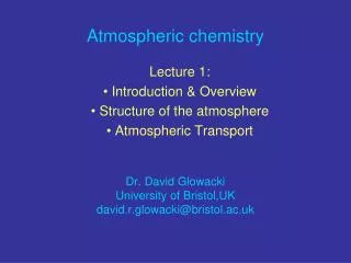
Lecture 16: Atmospheric chemistry • Questions • How do solar forcing, radiative and convective transfer set the vertical temperature structure of the atmosphere, the latitudinal heat transport by the atmosphere, and the global wind patterns that drive ocean circulation? • How does the greenhouse effect work? • What’s up with the ozone layer? • Tools • Gas phase chemistry, radiative and convective heat transfer, box models, photochemistry, etc. • Reading: • Grotzinger and Jordan Chapter 15 plus some issues raised in G & J chapter 23 • A good short book is Daniel Jacob, Introduction to Atmospheric Chemistry 1
Atmospheric structure: 0-D • Radiative forcing: the atmosphere is heated from above by UV absorption in stratosphere and from below by IR absorption in troposphere. Most sunlight (visible peak) gets through to the ground. A significant fraction (~75%) of the IR is absorbed and re-radiated at lower temperature. Outgoing radiation Incoming radiation 2
Atmospheric structure: 0-D • Radiative balance: incoming radiation = outgoing radiation • Incoming radiation = FSpr2(1- a) • Solar flux at 1 AU, FS = 1380 W/m2 • Area receiving sunlight is area of Earth projected as a disk, pr2, where r = 6471 km. • Albedo of earth a ~ 0.3 (where aice~1) • Outgoing radiation = 4pr2sTE4 • Area radiating is surface area of sphere, 4pr2 • TE is the effective blackbody temperature, s is the Stefan-Boltzmann constant • So TE = [FS(1- a) / 4s]1/4 = 255 K = –18 °C • So if the Surface temperature of the Earth were the effective radiating temperature (i.e., no atmosphere), all water would be frozen. • To raise TE to 273 K by lowering albedo alone would require a ≤ 0.08! 3
Atmospheric structure: Greenhouse effect I • Now imagine an atmospheric layer that is transparent to incoming solar radiation but absorbs a fraction f of outgoing infrared radiation. • Now we write two independent radiative balance equations, for the surface at temperature To and for the absorbing layer at T1 • Per unit area, FS(1- a)/4 = (1- f)sTo4 + fsT14 from space • Per unit area, 2fsT14 = fsTo4 at absorbing layer (top and bottom both radiate, hence the 2; we used Kirchhoff’s law el = al and a greybody assumption) • So To = [FS(1- a) / 4s(1-f/2)]1/4 and T1= To 2–1/4 • Hence actual mean ground temperature To = 288 K for the earth implies f = 0.77 (in which case T1 = 242 K). The maximum effect from a single layer would be at f = 1 and To = 304 K = 31 °C (in which case, naturally T1 = 255 K). Of course there could be different absorbing layers at different wavelengths, etc. 4
Atmospheric structure: Greenhouse effect II • Here is an actual outgoing radiation spectrum measured over Africa at noon. The ground is radiating at 320 K in the non-absorbing atmospheric window. The tropopause (where CO2 becomes optically thin) is radiating at ~215 K, the lower troposphere is radiating at ~270 K (H2O is thin above ~5 km). The stratosphere is radiating at 280 K (where O3 becomes optically thin) Of course, this is neither a steady-state nor a 0-dimensional situation, but in some sense the ground-atmosphere system must adjust itself to match the integral under this curve to incoming solar radiation 5
Atmospheric Structure: 1-D • Pressure structure • Hydrostatic equilibrium between pressure gradient and gravity • Ideal gas law (Ma = 28.96 g/mol) • Or, assuming constant T: • The logP-z curve in the figure is not quite linear because the temperature is not actually constant • Let H = RT/gMa be the scale height of the atmosphere (7.4 km at T=250 K): • Thus, e.g. a supersonic jet flying at 20 km is a full scale height above a normal jet flying at 12 km and sees ~1/e times the air density in its path 6
Atmospheric Structure: 1-D • Temperature structure • There are three reversals in the average temperature profile of the atmosphere that divide it into four layers: • The Thermosphere, above ~80 km (not shown in figure), gets very hot due to UV absorption by O2, but the density is so low it hardly matters • The Mesosphere is heated from below and has decreasing T with altitude • The stratosphere is heated from above by UV absorption by ozone. It is stably stratified. • The troposphere is heated by IR absorption by CO2 and H2O and may become convectively unstable. 9.8 K/km • Convective stability is defined by the temperature gradient relative to the adiabatic lapse rate. For dry air: a = 1/T for ideal gas • For saturated air, the moist lapse rate is more like 6 K/km 7
8 Atmospheric structure: 2-D • The Earth is unevenly heated by sunlight: the equator receives much more radiation per unit area than the poles • It is the job of the atmosphere and oceans to try to eliminate the resulting temperature gradient by zonal heat transport • The resulting transport is of two types: ocean transport is dominantly sensible heat transport (advection of warm water polewards), atmospheric transport is dominantly latent heat transport (low-latitude evaporation, high-latitude condensation)
Atmospheric structure: 2-D • Total zonal heat transport is obtained from radiative balance calculations based on solar forcing and measured outgoing IR as a function of latitude (see Problem Set 6) • Atmospheric heat transport is obtained from Radiosonde data that give abundant regular measurements of temperature, winds, and humidity • Oceanic heat transport is obtained by difference, but shows important features such as Western Boundary currents in North 9
Atmospheric structure: 3-D • In the absence of Coriolis force, solar forcing would drive single Hadley cells in each hemisphere, which we can understand using the “sea-breeze circulation” 10
Atmospheric structure: 3-D • But by ±30° latitude, the Coriolis force gets strong enough to break up the Hadley circulation, resulting in subtropical oceanic gyres, tropical rainfall, the 30° desert band, trade winds, etc. Remember the geostrophic equation? 11
Atmospheric structure: 3-D • But by ±30° latitude, the Coriolis force gets strong enough to break up the Hadley circulation, resulting in subtropical oceanic gyres, tropical rainfall, the 30° desert band, trade winds, etc. Remember the geostrophic equation? 12
Bulk chemistry of atmosphere • To first order, the modern atmosphere originated by degassing of volatile compounds from the earth’s interior. This process continues, as demonstrated for example by the 3He flux at mid-ocean ridges 13
Bulk chemistry of atmosphere • What comes out of the Earth: CO2, H2O, S, N2, noble gases • What is now in the atmosphere: • 78.08% N2 • 20.05% O2 • 0.9% Ar • 275 391 ppm CO2 • 0.0005% He • 0.00005% H2 • Why are they different? • H2O condenses. CO2 dissolves in oceans (60x more than atmosphere) and precipitates as carbonates. • Noble gas in atmosphere is dominantly radiogenic (40Ar, 4He) • H2 is lost from exosphere (He/H2 ratio ~ 10 is 1000x primordial ratio) • O2 is produced and maintained by biology 14
Geochemical cycles: Nitrogen • Here are the basic elements from which we might construct a box model to understand the cycling of Nitrogen in the surface reservoirs of the Earth: 15
Geochemical cycles: Nitrogen • Here is a steady-state quantification of the N box model: t = 13 Ma t = 0.03 a t = 27 a t = 0.6 a t = 4 a t = 50 a t = 200 Ma! 16
Geochemical cycles: Oxygen and Carbon • To make atmospheric oxygen, it is not enough to have photosynthesis, because respiration and decay of organic carbon take the oxygen back to CO2. • Rather, each mole of oxygen in the atmosphere must be compensated by a mole of buried organic C in sediments • But the total inventory of sedimentary organic C, about 107 Pg, is enough to account for 30 times the atmospheric inventory of O2! • Think about this next time you burn fossil fuel, but don’t think too hard…the industrial increase in CO2 from 280 to 380 ppm represents a decrease of O2 from 20 to 19.98% • The balance is accounted for by burial and storage of SO42- and Fe2O3, since the mantle provides mostly S2- and FeO. 17
Geochemical cycles: Carbon • The important greenhouse gases are CO2, CH4, and H2O (but H2O is a passive amplifier, not a cause), so global climate is intimately tied to the carbon cycle About this time Wally Broecker sent an alarmist letter to President Nixon about global cooling 18
Geochemical cycles: Carbon • Proxy records allow longer reconstructions than instrumental data... 19
Carbon • We have accurate measurements of the increase in atmospheric CO2 concentrations. • We can estimate the effect on climate forcing. • CO2 is the biggest climate forcing, but many others are significant. This is the 2001 assessment by the IPCC 20
Carbon • We also know from economic records the total amount of fossil fuel burned, and only about half the resulting CO2 has accumulated in the atmosphere…where is the rest? • Taken up by ocean and by terrestrial biosphere, but how much of each? • One good way to tell is from simultaneous high-precision data on O2 and CO2 • Fossil fuel, a mix of coal, gas, and oil, consumes 1.38 mol O2 for every 1 mol CO2 released • Land uptake by photosynthesis is 1:1, CO2+H2O=CH2O+O2 • Ocean uptake by solubility and pH adjustment has no effect on O2 • Ocean warming lowers O2 solubility, though 22
Stratospheric ozone: production and loss • The existence of ozone in the stratosphere determines the temperature structure of the upper atmosphere and, by the way, is essential for life at the Earth’s surface. • It is therefore worthwhile to understand the chemical kinetics of production and loss and the effects of anthropogenic gases. O3 photolysis O2 photolysis
Stratospheric ozone: production and loss • Production of ozone in the stratosphere is well understood; the mechanism was defined by Chapman in 1930: (activation reaction, l ≤ 240 nm, both oxygens are O(3P) ) (1) (M is any 3rd body; reactions 2 and 3 make a rapid cycle that defines the odd oxygen or Ox family, l ≤ 320 nm) (2) (3) (This O is O(1D) until some collision) (4) (quenching reaction) We will see that k2 and k3 are much greater than k1 and k4, so that at steady state there is a significant abundance of Ox and it does not matter whether it is O3 or O.
Stratospheric ozone: production and loss • Steady-state solution for ozone abundance: • Ox steady state means setting rate of reaction 2 equal to 3: where CO2 is the mixing ratio of O2 (0.2) and na is the number density of all air molecules (altitude dependent) • Then steady-state for entry and exit to Ox cycle means setting rate of reaction 1 equal to reaction 4: Note: the photolysis rate constants k1 and k3 include a term for the ultraviolet flux, so they increase upwards as the column depth of O2 and O3 above z decreases. On the other hand, the number density of the atmosphere falls off exponentially with increasing altitude.
Stratospheric ozone: production and loss Up here no O2 to react • Steady-state abundance of O3 depends on product of k1 and na3/2, so there is a maximum at ~30 km. The general shape of the prediction is a good match to abundance data. • But the Chapman mechanism predicts a factor of 2 too much O3…the source is certain so there must be another sink! Down here no UV flux
Stratospheric ozone: production and loss • The missing sinks for ozone come from catalytic loss cycles, i.e. reaction cycles where the ozone destruction agent is regenerated and can destroy many ozone molecules before it exits the cycle • Good catalysts are generally radical species with an odd number of electrons such as the hydroxyl radical OH (9 e–) • The OH loss cycle must be initiated by O(1D), normally produced by k3 photolysis of O3: Activation steps: removes one Ox, makes 2 OH, requires deep UV and H2O Catalytic cycle: net reaction is 2O3 -> 3O2(OH and OH2 are the HOx radical family) Termination step, slow
Stratospheric ozone: production and loss • The OH loss cycle is efficient in principle but does not account for enough O3 loss in the middle and upper stratosphere • Limited at low altitude by low UV flux • Limited at high altitude by very low H2O mixing ratio • A more important (but more complicated) natural catalytic loss cycle (whose discovery earned Paul Crutzen a Nobel prize) is the NOx radical system: NOx: radical species NO and NO2 NOy: nonradical reservoir species N2O5 and HNO3
Stratospheric ozone: production and loss • When reaction of NO with O3 produces NO2, it has several possible fates: • Photolysis cycles it back to NO with no net effect • Reaction with O catalytically destroys two Ox species • Reaction with OH radical or O3 inactivates one NOx NOx cycle: no net effect, but rapidly cycles NO & NO2 Catalytic cycle branch: net reaction consumes 2 Ox Termination step, daytime Termination step, nighttime
Stratospheric ozone: production and loss • Because N2O from the biosphere is stable and non-condensable, it reaches upper stratosphere and meets enough O(1D) to form NOx and initiate O3-loss catalysis • The other O3-loss mechanism is mostly anthropogenic and involves sources of Cl and Br stable enough to reach stratosphere Together, the Chapman source roughly balances these four loss mechanisms and explains the O3 abundance at all heights in the normal stratosphere: Chapman (O3+O), HOx, NOx, and ClOx
Polar Stratospheric ozone: the Antarctic Ozone Hole • The total disappearance of the ozone layer in the mid-stratosphere over Antarctica provides a challenge to the standard gas-phase theory of ozone balance, since in winter there is not enough light to drive the HOx, NOx, or ClOx losses October 2000 October 2002: ?
Polar Stratospheric ozone: the Antarctic Ozone Hole The story is complicated but here is its essence: 1) When temperature drops below 197 K Polar Stratospheric Clouds (PSC) of HNO3•3H2O can form even though H2O is very rare. 2) PSC surfaces provide rapid total conversion of inactive Cl species HCl and ClNO3 to active ClOx and HNO3. 3) When temperatures rise again in September, the HNO3 would scavenge all the ClOx back to ClNO3, except that the PSC particles grow big enough to sediment out of the stratosphere, removing HNO3 and leaving behind active ClOx. 4) When light returns in Southern Spring, at high ClO concentrations a catalytic photolysis mechanism can run that consumes O3 without O(1D). (More Nobel-quality chemistry, this time to Molina and Rowland)
Tropospheric Ozone • Yes, the air in Pasadena really is getting better! 34