Download
1 / 47
470 likes | 602 Views
A Doppler Radar Emulator and its Application to the Detection of Tornadic Signatures. Ryan M. May. Acknowledgements. Reading Committee Dr. Michael Biggerstaff Dr. Ming Xue Dr. Robert Palmer Dr. Tian-You Yu Curtis Alexander Gordon Carrie. Motivation.

E N D
A Doppler Radar Emulator and its Application to the Detection of Tornadic Signatures Ryan M. May
Acknowledgements • Reading Committee • Dr. Michael Biggerstaff • Dr. Ming Xue • Dr. Robert Palmer • Dr. Tian-You Yu • Curtis Alexander • Gordon Carrie
Motivation • Create tool that generates radar moment data for a given set of radar operating parameters • Useful for: • Radar system design • Scanning strategy design • Algorithm development • Retrieval technique evaluation
Previous Work • Zrnic (1975) simulated time series radar data using an assumed Gaussian distribution of velocities within a volume • Chandrasekar and Bringi (1987) simulated reflectivity values as a function of raindrop size distribution parameters • Wood and Brown (1997) evaluated the effects of WSR-88D scanning strategies on the sampling of mesocyclones and tornadoes • Capsoni and D’Amico (1998) simulated time series radar data using returns from individual hydrometeors within a volume
Radar Configuration • Pulse Length • PRF • Pulses per Radial • Rotation Rate • Gate Length • Scan Angles • Wavelength • Location • Transmit Power • Antenna Gain • Antenna Beamwidth • Noise Threshold
Capabilities • Azimuthal Resolution • Range Resolution • Attenuation • Range Aliasing • Velocity Aliasing • Anomalous Propagation • Antenna Sidelobes
Scattering • Currently, the Rayleigh approximation is used for scattering: • Rain is assumed to have a Marshall-Palmer distribution • Cloud droplets are assumed to be monodisperse
Emulator Design • A “pulse” is propagated through the model’s numerical output grid along the current pointing angle • This pulse is subdivided into many small, individual elements • Each element is assigned values for reflectivity, radial velocity, and attenuation factor from the model grid, using nearest neighbor sampling
Emulator Design (cont.) Representation of segmented pulse being matched to model grid field
Emulator Design (cont.) • At a given instant, two pulses are being used, allowing for the simulation of 2nd trip echoes • For every range gate along the beam, the pulses are sampled to produce a value of returned power, Doppler velocity, and velocity variance
Emulator Design (cont.) • Returned power is calculated as: • Doppler velocity is the power-weighted average of all velocities for all pulse elements • The velocity variance for the pulse is the power-weighted variance of velocities for all pulse elements
Emulator Design (cont.) • When the returns for the specified number of pulses for a radial have been calculated, a radial of data is generated • Returned power is the average returned power for all pulses • Doppler velocity is the power-weighted average velocity for all pulses • Spectrum width is the power-weighted variance for all pulses
Emulator Design (cont.) • At this point, the velocity is forced to a value within the Nyquist co-interval, simulating velocity aliasing • Also, equivalent radar reflectivity factor is calculated from the returned power as:
Simulation Characteristics • Simulation created using the Advanced Regional Prediction System (ARPS) • Horizontal grid resolution: 50m • Stretched vertical grid (~18m at surface) • Warm rain precipitation microphysics • Produces a 200m diameter tornado with a 160 m/s change in velocity across the vortex
ARPS Simulation Vector Velocity, Rain Water Mixing Ratio, and Total Buoyancy
Examples – 10cm, 1o Beamwidth Equivalent Reflectivity Factor Returned Power Doppler Velocity Spectrum Width
Examples – Azimuthal Oversampling CONTROL Equivalent Reflectivity Factor CONTROL Doppler Velocity OVERSAMPLEDEquivalent Reflectivity Factor OVERSAMPLED Doppler Velocity
Examples – Azimuthal Oversampling Equivalent Reflectivity Factor Difference (Oversampled - Orginal)
Examples – 125m Gate Spacing CONTROL Equivalent Reflectivity Factor CONTROL Doppler Velocity 125M GATE SPACING Doppler Velocity 125M GATE SPACING Equivalent Reflectivity Factor
Examples – No Sidelobes CONTROL Equivalent Reflectivity Factor CONTROL Doppler Velocity NO SIDELOBES Equivalent Reflectivity Factor NO SIDELOBES Doppler Velocity
Examples – No Sidelobes Returned Power Difference (Original – No Sidelobes)
Examples – 2o Beamwidth Equivalent Reflectivity Factor (original) Doppler Velocity (original) Equivalent Reflectivity Factor (2o Beamwidth) Doppler Velocity (2o Beamwidth)
Examples – Low PRF Equivalent Reflectivity Factor Returned Power Doppler Velocity Spectrum Width
Examples – X-band (3cm) Equivalent Reflectivity Factor Returned Power Doppler Velocity Spectrum Width
Examples – X-band (3cm) Returned Power Difference (Original – X-band)
Examples – 2nd Trip Echoes Equivalent Reflectivity Factor Returned Power Doppler Velocity Spectrum Width
From Examples to Application • We’ve now seen examples of the emulator’s capabilities • Let’s move on to material that’s more…practical: detecting tornadoes
Example Application:Tornado Detection • Emulated data for prototype CASA radars • 4 Metrics for tornado intensity: • Maximum velocity • ΔVelocity • Diameter • Axisymmetric vorticity: 2ΔV / D • 4 Ranges : 3km, 10km, 30km, 50km • Matched Sampling / Oversampling
Tornado – 3km, Matched Sampling Spectrum Width Equivalent Reflectivity Factor Doppler Velocity Doppler Velocity (no aliasing)
Tornado – 3km, Oversampling Spectrum Width Equivalent Reflectivity Factor Doppler Velocity Doppler Velocity (no aliasing)
Tornado – 10km, Matched Sampling Spectrum Width Equivalent Reflectivity Factor Doppler Velocity Doppler Velocity (no aliasing)
Tornado – 10km, Oversampling Spectrum Width Equivalent Reflectivity Factor Doppler Velocity Doppler Velocity (no aliasing)
Tornado – 30km, Matched Sampling Spectrum Width Equivalent Reflectivity Factor Doppler Velocity Doppler Velocity (no aliasing)
Tornado – 30km, Oversampling Spectrum Width Equivalent Reflectivity Factor Doppler Velocity Doppler Velocity (no aliasing)
Tornado – 50km, Matched Sampling Spectrum Width Equivalent Reflectivity Factor Doppler Velocity Doppler Velocity (no aliasing)
Tornado – 50km, Oversampling Spectrum Width Equivalent Reflectivity Factor Doppler Velocity Doppler Velocity (no aliasing)
Conclusions • The large beamwidth of the CASA radars will be significant hurdle to the detection of tornadoes • Oversampling does help mitigate some of this problem • These sampling issues will compound the dealiasing problems due to the low Nyquist velocity at X-band • The quality of the dealiasing procedure for the data will be extremely important
Future Studies • Continue examining the detectability of tornadoes • Test detection using objective algorithms • Examine impacts of attenuation • Examine data for times when storm is not tornadic • Examine vertical continuity • Evaluate scanning impacts on quality of dual Doppler analysis
Future Development • Mie Scattering • Phased Array Antenna • Time Evolution of Model Field • Polarimetric Variables • Ground Clutter Targets
Questions? Capsoni, C., and M. D'Amico, 1998: A physically based radar simulator. J. Atmos. Oceanic Technol., 15, 593-598. Chandrasekar, V., and V. N. Bringi, 1987: Simulation of radar reflectivity and surface measurements of rainfall. J. Atmos. Oceanic Technol., 4, 464-478. Wood, V. T., and R. A. Brown, 1997: Effects of radar sampling on single-Doppler velocity signatures of mesocyclones and tornadoes. Wea. Forecasting, 12, 928-938. Zrnic, D. S., 1975: Simulation of weatherlike Doppler spectra and signals. J. App. Meteor.,14, 619-620.
Examples – 10cm, 1o Beamwidth Equivalent Reflectivity Factor Returned Power Doppler Velocity Spectrum Width
Examples – 125m Gate Spacing Equivalent Reflectivity Factor Returned Power (control) Doppler Velocity Spectrum Width
Examples – No Sidelobes Equivalent Reflectivity Factor Returned Power Doppler Velocity Spectrum Width
Examples – 2o Beamwidth Equivalent Reflectivity Factor Returned Power Doppler Velocity Spectrum Width