Download
1 / 20
200 likes | 323 Views
This document delves into the modeling of acoustic impedance and boundary effects related to the vocal tract. It analyzes the assumptions about pressure at the lips, the ideal volume velocity source, and energy loss. Key studies including Morse and Ingard (1986), Flanagan (1972), and others are referenced to explain lip radiation modeled as a piston in an infinite wall. The resulting physics illustrates how resonances shift due to various losses, and how bandwidths of resonances are influenced by wall vibration, glottal impedance, and radiation losses in concatenated tube models.

E N D
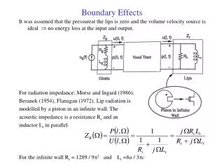
Boundary Effects It was assumed that the pressureat the lips is zero and the volume velocity source is ideal no energy loss at the input and output. For radiation impedance: Morse and Ingard (1986), Beranek (1954), Flanagan (1972). Lip radiation is modelled by a piston in an infinite wall. The acoustic impedance is a resistance Rr and an inductor Lr in parallel. For the infinite wall Rr = 1289 / 92 and Lr =8a / 3c
Boundary Effects The impedance equation can be converted to a differential equation via Laplace transform. Portnoff (1973) numerically simulated the above equation coupled to the wave equation. Broader bandwidths and lowering of the resonances are observed. Higher frequencies are affected most. (This can be seen by considering Zr 0 when 0 (small) p(l,t) = 0 but for large , Lr >>Rr Zr = Rr)
Glottal Source and Impedance Flanagan-Isızaka (1978) proposed a linear model for the impedance. This is a differential equation in the time-domain. The solution of this equation together with the wave equation yields broadening of the bandwidths at low frequencies. This can be seen from Zg = Rg + j Lg becomes ZgRg for small ; (purely resistive). Overall Frequency Response introduces a highpass filter effect
Summarizing the results • Resonances are due to vocal tract. Resonant frequenciesshift as a result various losses. • Bandwidths of lower resonances are controlledby wall vibration and glottal impedance loss. • Bandwidths of higher resonances are controlled by radiation, viscous and thermal losses.
Model of Concatenated Tubes (Energy loss is assumed to be only at the lips.) For the kth tube (*) Boundary conditions are
Model of Concatenated Tubes The boundary conditions and (*) yield : Let k=lk /c Using in (2)
Model of Concatenated Tubes (4) – (3) Let Both equations contain a component due to reflection and one component due to transmission.
Boundary Relations Lips: Suppose radiation impedance is real. At the Nth tube Since There is no backward going wave from free space.
Boundary Relations Therefore Outgoing wave from the lips: Let the outer space be represented by an infinite length tube of cross section AN+1 , and in particular, if (Also, if Zr () = 0 rL=1, AN+1 no radiation from the lips.
Boundary Relations Glottis: Suppose the glottal impedance is purely real, Zg=Rg In particular, if glottal impedance is modeled by a tube of cross section A0 and A0 is chosen such that By chosig Ak s properly it is possible to approximate formant bandwidths.
Discrete Time Realization Consider a vocal-tract model consisting of N lossless concatenated tubes with total length l. length of a tube = x = l/N propagation time in a tube = = x/c Let va(t) be the impulse samples of the impulse response with 2 intervals. At the end of the tube va(t) can be written as: Since the samples up to time N will be zero. The Laplace transform and the frequency response are The frequency response is periodic with 2/2; Va(+ 2/2) = Va()
Discrete Time Realization If the impulse response of the system is not band limited then aliasing will occur. The discrete-time frequency response can be obtained by = /2
Discrete Time Realization The effect of aliasing can be reduced by decreasing the individual tube lengths and hence the sampling period. It can be shown that the transfer function of the discrete-time model has the form When Ak > 0 all poles are inside the unit circle.
Discrete Time Realization Ex: Let l=17.5 cm, c=350 m/sec. Find N to cover a bandwidth of 5000 Hz. (Assume that vocal tract impulse response and excitation are bandlimited to 5000 Hz.) Soln: /2 is the cutoff bandwidth. 5000 Hz 10000 rad/sec /2 = 10000 = 1/20000 N = l/c = 10 Since N is the order of the system, there are 5 complex conjugate poles There can be 5 resonances in the given bandwidth.
Discrete Time Realization Comparison of numerical simulation of differential equations and concatenated tube model (N=10) Tube cross sections Reflection coefficients
Simulation Concatenated tubes