BAYESIAN NETWORK
BAYESIAN NETWORK. Submitted By Faisal Islam Srinivasan Gopalan Vaibhav Mittal Vipin Makhija Prof. Anita Wasilewska State University of New York at Stony Brook. References. [ 1]Jiawei Han: ” Data Mining Concepts and Techniques ” ,ISBN 1-53860-489-8 Morgan Kaufman Publisher.

BAYESIAN NETWORK
E N D
Presentation Transcript
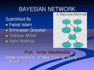
BAYESIAN NETWORK Submitted By • Faisal Islam • Srinivasan Gopalan • Vaibhav Mittal • Vipin Makhija Prof. Anita Wasilewska State University of New York at Stony Brook
References • [1]Jiawei Han:”Data Mining Concepts and Techniques”,ISBN 1-53860-489-8 Morgan Kaufman Publisher. • [2] Stuart Russell,Peter Norvig “Artificial Intelligence – A modern Approach ,Pearson education. • [3] Kandasamy,Thilagavati,Gunavati , Probability, Statistics and Queueing Theory , Sultan Chand Publishers. • [4] D. Heckerman: “A Tutorial on Learning with Bayesian Networks”, In “Learning in Graphical Models”, ed. M.I. Jordan, The MIT Press, 1998. • [5] http://en.wikipedia.org/wiki/Bayesian_probability • [6] http://www.construction.ualberta.ca/civ606/myFiles/Intro%20to%20Belief%20Network.pdf • [7] http://www.murrayc.com/learning/AI/bbn.shtml • [8] http://www.cs.ubc.ca/~murphyk/Bayes/bnintro.html • [9] http://en.wikipedia.org/wiki/Bayesian_belief_network
CONTENTS • HISTORY • CONDITIONAL PROBABILITY • BAYES THEOREM • NAÏVE BAYES CLASSIFIER • BELIEF NETWORK • APPLICATION OF BAYESIAN NETWORK • PAPER ON CYBER CRIME DETECTION
HISTORY • Bayesian Probability was named after Reverend Thomas Bayes (1702-1761). • He proved a special case of what is currently known as the Bayes Theorem. • The term “Bayesian” came into use around the 1950’s. • Pierre-Simon, Marquis de Laplace (1749-1827) independently proved a generalized version of Bayes Theorem. http://en.wikipedia.org/wiki/Bayesian_probability
HISTORY (Cont.) • 1950’s – New knowledge in Artificial Intelligence • 1958 Genetic Algorithms by Friedberg (Holland and Goldberg ~1985) • 1965 Fuzzy Logic by Zadeh at UC Berkeley • 1970 Bayesian Belief Network at Stanford University (Judea Pearl 1988) • The idea’s proposed above was not fully developed until later. BBN became popular in the 1990s. http://www.construction.ualberta.ca/civ606/myFiles/Intro%20to%20Belief%20Network.pdf
HISTORY (Cont.) Current uses of Bayesian Networks: • Microsoft’s printer troubleshooter. • Diagnose diseases (Mycin). • Used to predict oil and stock prices • Control the space shuttle • Risk Analysis – Schedule and Cost Overruns.
CONDITIONAL PROBABILITY • Probability : How likely is it that an event will happen? • Sample Space S • Element of S: elementary event • An event A is a subset of S • P(A) • P(S) = 1 Events A and B • P(A|B)- Probability that event A occurs given that event B has already occurred. Example: There are 2 baskets. B1 has 2 red ball and 5 blue ball. B2 has 4 red ball and 3 blue ball. Find probability of picking a red ball from basket 1?
CONDITIONAL PROBABILITY • The question above wants P(red ball | basket 1). • The answer intuitively wants the probability of red ball from only the sample space of basket 1. • So the answer is 2/7 • The equation to solve it is: P(A|B) = P(A∩B)/P(B) [Product Rule] P(A,B) = P(A)*P(B) [ If A and B are independent ] How do you solve P(basket2 | red ball) ???
BAYESIAN THEOREM • A special case of Bayesian Theorem: P(A∩B) = P(B) x P(A|B) P(B∩A) = P(A) x P(B|A) Since P(A∩B) = P(B∩A), P(B) x P(A|B) = P(A) x P(B|A) => P(A|B) = [P(A) x P(B|A)] / P(B) A B
BAYESIAN THEOREM Solution to P(basket2 | red ball) ? P(basket 2| red ball) = [P(b2) x P(r | b2)] / P(r) = (1/2) x (4/7)] / (6/14) = 0.66
BAYESIAN THEOREM • Example 2: A medical cancer diagnosis problem There are 2 possible outcomes of a diagnosis: +ve, -ve. We know .8% of world population has cancer. Test gives correct +ve result 98% of the time and gives correct –ve result 97% of the time. If a patient’s test returns +ve, should we diagnose the patient as having cancer?
BAYESIAN THEOREM P(cancer) = .008 P(-cancer) = .992 P(+ve|cancer) = .98 P(-ve|cancer) = .02 P(+ve|-cancer) = .03 P(-ve|-cancer) = .97 Using Bayes Formula: P(cancer|+ve) = P(+ve|cancer)xP(cancer) / P(+ve) = 0.98 x 0.008 = .0078 / P(+ve) P(-cancer|+ve) = P(+ve|-cancer)xP(-cancer) / P(+ve) = 0.03 x 0.992 = 0.0298 / P(+ve) So, the patient most likely does not have cancer.
BAYESIAN THEOREM • General Bayesian Theorem: Given E1, E2,…,En are mutually disjoint events and P(Ei) ≠ 0, (i = 1, 2,…, n) P(Ei/A) = [P(Ei) x P(A|Ei)] / Σ P(Ei) x P(A|Ei) i = 1, 2,…, n
BAYESIAN THEOREM • Example: There are 3 boxes. B1 has 2 white, 3 black and 4 red balls. B2 has 3 white, 2 black and 2 red balls. B3 has 4 white, 1 black and 3 red balls. A box is chosen at random and 2 balls are drawn. 1 is white and other is red. What is the probability that they came from the first box??
BAYESIAN THEOREM Let E1, E2, E3 denote events of choosing B1, B2, B3 respectively. Let A be the event that 2 balls selected are white and red. P(E1) = P(E2) = P(E3) = 1/3 P(A|E1) = [2c1 x 4c1] / 9c2 = 2/9 P(A|E2) = [3c1 x 2c1] / 7c2 = 2/7 P(A|E3) = [4c1 x 3c1] / 8c2 = 3/7
BAYESIAN THEOREM P(E1|A) = [P(E1) x P(A|E1)] / Σ P(Ei) x P(A|Ei) = 0.23727 P(E2|A) = 0.30509 P(E3|A) = 1 – (0.23727 + 0.30509) = 0.45764
BAYESIAN CLASSIFICATION Why use Bayesian Classification: • Probabilistic learning: Calculate explicit probabilities for hypothesis, among the most practical approaches to certain types of learning problems • Incremental: Each training example can incrmentally increase/decrease the probability that a hypothesis is correct. Prior knowledge can be combined with observed data.
BAYESIAN CLASSIFICATION • Probabilistic prediction: Predict multiple hypotheses, weighted by their probabilities • Standard: Even when Bayesian methods are computationally intractable, they can provide a standard of optimal decision making against which other methods can be measured
NAÏVE BAYES CLASSIFIER • A simplified assumption: attributes are conditionally independent: • Greatly reduces the computation cost, only count the class distribution.
NAÏVE BAYES CLASSIFIER The probabilistic model of NBC is to find the probability of a certain class given multiple dijoint (assumed) events. The naïve Bayes classifier applies to learning tasks where each instance x is described by a conjunction of attribute values and where the target function f(x) can take on any value from some finite set V. A set of training examples of the target function is provided, and a new instance is presented, described by the tuple of attribute values <a1,a2,…,an>. The learner is asked to predict the target value, or classification, for this new instance.
NAÏVE BAYES CLASSIFIER Abstractly, probability model for a classifier is a conditional model P(C|F1,F2,…,Fn) Over a dependent class variable C with a small nuumber of outcome or classes conditional over several feature variables F1,…,Fn. Naïve Bayes Formula: P(C|F1,F2,…,Fn) = argmaxc [P(C) x P(F1|C) x P(F2|C) x…x P(Fn|C)] / P(F1,F2,…,Fn) Since P(F1,F2,…,Fn) is common to all probabilities, we donot need to evaluate the denomitator for comparisons.
NAÏVE BAYES CLASSIFIER Tennis-Example
NAÏVE BAYES CLASSIFIER • Problem: Use training data from above to classify the following instances: • <Outlook=sunny, Temperature=cool, Humidity=high, Wind=strong> • <Outlook=overcast, Temperature=cool, Humidity=high, Wind=strong>
NAÏVE BAYES CLASSIFIER Answer to (a): P(PlayTennis=yes) = 9/14 = 0.64 P(PlayTennis=n) = 5/14 = 0.36 P(Outlook=sunny|PlayTennis=yes) = 2/9 = 0.22 P(Outlook=sunny|PlayTennis=no) = 3/5 = 0.60 P(Temperature=cool|PlayTennis=yes) = 3/9 = 0.33 P(Temperature=cool|PlayTennis=no) = 1/5 = .20 P(Humidity=high|PlayTennis=yes) = 3/9 = 0.33 P(Humidity=high|PlayTennis=no) = 4/5 = 0.80 P(Wind=strong|PlayTennis=yes) = 3/9 = 0.33 P(Wind=strong|PlayTennis=no) = 3/5 = 0.60
NAÏVE BAYES CLASSIFIER P(yes)xP(sunny|yes)xP(cool|yes)xP(high|yes)xP(strong|yes) = 0.0053 P(no)xP(sunny|no)xP(cool|no)xP(high|no)x P(strong|no) = 0.0206 So the class for this instance is ‘no’. We can normalize the probility by: [0.0206]/[0.0206+0.0053] = 0.795
NAÏVE BAYES CLASSIFIER Answer to (b): P(PlayTennis=yes) = 9/14 = 0.64 P(PlayTennis=no) = 5/14 = 0.36 P(Outlook=overcast|PlayTennis=yes) = 4/9 = 0.44 P(Outlook=overcast|PlayTennis=no) = 0/5 = 0 P(Temperature=cool|PlayTennis=yes) = 3/9 = 0.33 P(Temperature=cool|PlayTennis=no) = 1/5 = .20 P(Humidity=high|PlayTennis=yes) = 3/9 = 0.33 P(Humidity=high|PlayTennis=no) = 4/5 = 0.80 P(Wind=strong|PlayTennis=yes) = 3/9 = 0.33 P(Wind=strong|PlayTennis=no) = 3/5 = 0.60
NAÏVE BAYES CLASSIFIER Estimating Probabilities: In the previous example, P(overcast|no) = 0 which causes the formula- P(no)xP(overcast|no)xP(cool|no)xP(high|no)xP(strong|nno) = 0.0 This causes problems in comparing because the other probabilities are not considered. We can avoid this difficulty by using m- estimate.
NAÏVE BAYES CLASSIFIER M-Estimate Formula: [c + k] / [n + m] where c/n is the original probability used before, k=1 and m= equivalent sample size. Using this method our new values of probility is given below-
NAÏVE BAYES CLASSIFIER New answer to (b): P(PlayTennis=yes) = 10/16 = 0.63 P(PlayTennis=no) = 6/16 = 0.37 P(Outlook=overcast|PlayTennis=yes) = 5/12 = 0.42 P(Outlook=overcast|PlayTennis=no) = 1/8 = .13 P(Temperature=cool|PlayTennis=yes) = 4/12 = 0.33 P(Temperature=cool|PlayTennis=no) = 2/8 = .25 P(Humidity=high|PlayTennis=yes) = 4/11 = 0.36 P(Humidity=high|PlayTennis=no) = 5/7 = 0.71 P(Wind=strong|PlayTennis=yes) = 4/11 = 0.36 P(Wind=strong|PlayTennis=no) = 4/7 = 0.57
NAÏVE BAYES CLASSIFIER P(yes)xP(overcast|yes)xP(cool|yes)xP(high|yes)xP(strong|yes) = 0.011 P(no)xP(overcast|no)xP(cool|no)xP(high|no)xP(strong|nno) = 0.00486 So the class of this instance is ‘yes’
NAÏVE BAYES CLASSIFIER • The conditional probability values of all the attributes with respect to the class are pre-computed and stored on disk. • This prevents the classifier from computing the conditional probabilities every time it runs. • This stored data can be reused to reduce the latency of the classifier.
BAYESIAN BELIEF NETWORK • In Naïve Bayes Classifier we make the assumption of class conditional independence, that is given the class label of a sample, the value of the attributes are conditionally independent of one another. • However, there can be dependences between value of attributes. To avoid this we use Bayesian Belief Network which provide joint conditional probability distribution. • A Bayesian network is a form of probabilistic graphical model. Specifically, a Bayesian network is a directed acyclic graph of nodes representing variables and arcs representing dependence relations among the variables.
BAYESIAN BELIEF NETWORK • A Bayesian network is a representation of the joint distribution over all the variables represented by nodes in the graph. Let the variables be X(1), ..., X(n). • Let parents(A) be the parents of the node A. Then the joint distribution for X(1) through X(n) is represented as the product of the probability distributions P(Xi|Parents(Xi)) for i = 1 to n. If X has no parents, its probability distribution is said to be unconditional, otherwise it is conditional.
BAYESIAN BELIEF NETWORK • By the chaining rule of probability, the joint probability of all the nodes in the graph above is: P(C, S, R, W) = P(C) * P(S|C) * P(R|C) * P(W|S,R) W=Wet Grass, C=Cloudy, R=Rain, S=Sprinkler Example: P(W∩-R∩S∩C) = P(W|S,-R)*P(-R|C)*P(S|C)*P(C) = 0.9*0.2*0.1*0.5 = 0.009
BAYESIAN BELIEF NETWORK What is the probability of wet grass on a given day - P(W)? P(W) = P(W|SR) * P(S) * P(R) + P(W|S-R) * P(S) * P(-R) + P(W|-SR) * P(-S) * P(R) + P(W|-S-R) * P(-S) * P(-R) Here P(S) = P(S|C) * P(C) + P(S|-C) * P(-C) P(R) = P(R|C) * P(C) + P(R|-C) * P(-C) P(W)= 0.5985
Advantages of Bayesian Approach • Bayesian networks can readily handle incomplete data sets. • Bayesian networks allow one to learn about causal relationships • Bayesian networks readily facilitate use of prior knowledge.
Sources/References • Naive Bayes Spam Filtering Using Word-Position-Based Attributes- http://www.ceas.cc/papers-2005/144.pdf by-: Johan Hovold, Department of Computer Science,Lund University Box 118, 221 00 Lund, Sweden.[E-mail johan.hovold.363@student.lu.se] [Presented at CEAS 2005 Second Conference on Email and Anti-SpamJuly 21 & 22, at Stanford University] • Tom Mitchell , “ Machine Learning” , Tata Mcgraw Hill • A Bayesian Approach to Filtering Junk EMail, Mehran Sahami Susan Dumaisy David Heckermany Eric Horvitzy Gates Building Computer Science Department Microsoft Research, Stanford University Redmond W Stanford CA fsdumais heckerma horvitzgmicrosoftcom [Presented at AAAI Workshop on Learning for Text Categorization, July 1998, Madison, Wisconsin]
Problem??? • real world Bayesian network application – “Learning to classify text. “ • Instances are text documents • we might wish to learn the target concept “electronic news articles that I find interesting,” or “pages on the World Wide Web that discuss data mining topics.” • In both cases, if a computer could learn the target concept accurately, it could automatically filter the large volume of online text documents to present only the most relevant documents to the user.
TECHNIQUE • learning how to classify text, based on the naive Bayes classifier • it’s a probabilistic approach and is among the most effective algorithms currently known for learning to classify text documents, • Instance space X consists of all possible text documents • given training examples of some unknown target function f(x), which can take on any value from some finite set V • we will consider the target function classifying documents as interesting or uninteresting to a particular person, using the target values like and dislike to indicate these two classes.
Design issues • how to represent an arbitrary text document in terms of attribute values • decide how to estimate the probabilities required by the naive Bayes classifier
Approach • Our approach to representing arbitrary text documents is disturbingly simple: Given a text document, such as this paragraph, we define an attribute for each word position in the document and define the value of that attribute to be the English word found in that position. Thus, the current paragraph would be described by 111 attribute values, corresponding to the 111 word positions. The value of the first attribute is the word “our,” the value of the second attribute is the word “approach,” and so on. Notice that long text documents will require a larger number of attributes than short documents. As we shall see, this will not cause us any trouble.
ASSUMPTIONS • assume we are given a set of 700 training documents that a friend has classified as dislike and another 300 she has classified as like • We are now given a new document and asked to classify it • let us assume the new text document is the preceding paragraph
We know (P(like) = .3 and P (dislike) = .7 in the current example P(ai , = wk|vj) (here we introduce wkto indicate the kth word in the English vocabulary) estimating the class conditional probabilities (e.g., P(ai= “our”Idislike)) is more problematic because we must estimate one such probability term for each combination of text position, English word, and target value. there are approximately 50,000 distinct words in the English vocabulary, 2 possible target values, and 111 text positions in the current example, so we must estimate 2*111* 50, 000 =~10 million such terms from the training data. we make assumption that reduces the number of probabilities that must be estimated
we shall assume the probability of encountering a specific word wk(e.g., “chocolate”) is independent of the specific word position being considered (e.g., a23 versus a95) . • we estimate the entire set of probabilities P(a1= wk|vj), P(a2= wk|vj)... by the single position-independent probability P(wklvj) • net effect is that we now require only 2* 50, 000 distinct terms of the form P(wklvj) • We adopt the rn-estimate, with uniform priors and with m equal to the size of the word vocabulary • n total number of word positions in all training examples whose target value is v, nkis the number of times word Wkis found among these n word positions, and Vocabulary is the total number of distinct words (and other tokens) found within the training data.
Final Algorithm • Examples is a set of text documents along with their target values. V is the set of all possible target values. This function learns the probability terms P( wk| vj), describing the probability that a randomly drawn word from a document in class vj will be the English word Wk. It also learns the class prior probabilities P(vi). 1. collect all words, punctuation, and other tokens that occur in Examples • Vocabulary set of all distinct words & tokens occurring in any text document from Examples 2. calculate the required P(vi) and P( wk| vj) probability terms • For each target value vj in V do • docsj the subset of documents from Examples for which the target value is vj• P(v1) IdocsjI / \Examplesl • Textja single document created by concatenating all members of docsj• n total number of distinct word positions in Textj• for each word Wkin Vocabulary nknumber of times word wkoccurs in Textj• P(wkIvj) nk+1/n+|Vocabulary| CLASSIFY_NAIVE_BAYES_TEXT( Doc) Return the estimated target value for the document Doc. ai denotes the word found in the ith position within Doc. • positions all word positions in Doc that contain tokens found in Vocabulary • Return VNB, where
During learning, the procedure LEARN_NAIVE_BAYES_TEXT examines all training documents to extract the vocabulary of all words and tokens that appear in the text, then counts their frequencies among the different target classes to obtain the necessary probability estimates. Later, given a new document to be classified, the procedure CLASSIFY_NAIVE_BAYESTEXT uses these probability estimates to calculate VNB according to Equation Note that any words appearing in the new document that were not observed in the training set are simply ignored by CLASSIFY_NAIVE_BAYESTEXT
Effectiveness of the Algorithm • Problem classifying usenet news articles • target classification for an article name of the usenet newsgroup in which the article appeared • In the experiment described by Joachims (1996), 20 electronic newsgroups were considered • 1,000 articles were collected from each newsgroup, forming a data set of 20,000 documents. The naive Bayes algorithm was then applied using two-thirds of these 20,000 documents as training examples, and performance was measured over the remaining third. • 100 most frequent words were removed (these include words such as “the” and “of’), and any word occurring fewer than three times was also removed. The resulting vocabulary contained approximately 38,500 words. • The accuracy achieved by the program was 89%.

