Categorical Data
Categorical Data. Ziad Taib Biostatistics AstraZeneca February 2014. Types of Data. Continuous Blood pressure Time to event. Categorical sex. quantitative. qualitative. Discrete No of relapses. Ordered Categorical Pain level. Types of data analysis (Inference). Parametric Vs

Categorical Data
E N D
Presentation Transcript
Categorical Data ZiadTaib Biostatistics AstraZeneca February 2014
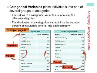
Types of Data Continuous Blood pressure Time to event Categorical sex quantitative qualitative Discrete No of relapses Ordered Categorical Pain level
Types of data analysis (Inference) Parametric Vs Non parametric Model based Vs Data driven Frequentist Vs Bayesian
Categorical data In a RCT, endpoints and surrogate endpoints can be categorical or ordered categorical variables. In the simplest cases we have binary responses (e.g. responders non-responders). In Outcomes research it is common to use many ordered categories (no improvement, moderate improvement, high improvement).
Binary variables • Sex • Mortality • Presence/absence of an AE • Responder/non-responder according to some pre-defined criteria • Success/Failure
Inference problems • Binary data (proportions) • One sample • Paired data • Ordered categorical data • Combining categorical data • Logistic regression • A Bayesian alternative • ODDS and NNT
Categorical data In a RCT, endpoints and surrogate endpoints can be categorical or ordered categorical variables. In the simplest cases we have binary responses (e.g. responders non-responders). In Outcomes research it is common to use many ordered categories (no improvement, moderate improvement, high improvement).
Bernoulli experiment Success1 With probability p Random experience Failure0 Hole in one? With probability1-p
Binary variables • Sex • Mortality • Presence/absence of an AE • Responder/non-responder according to some pre-defined criteria • Success/Failure
Estimation • Assume that a treatment has been applied to n patients and that at the end of the trial they were classified according to how they responded to the treatment: 0 meaning not cured and 1 meaning cured. The data at hand is thus a sample of n independent binary variables • The probability of being cured by this treatment can be estimated by satisfying
Hypothesis testing • We can test the null hypothesis • Using the test statistic • When n is large, Z follows, under the null hypothesis, the standard normal distribution (obs! Not when p very small or very large).
Hypothesis testing • For moderate values of n we can use the exact Bernoulli distribution of leading to the sum being Binomially distributed i.e. • As with continuous variables, tests can be used to build confidence intervals.
Example 1: Hypothesis test based on binomial distr. Consider testing H0: P=0.5 against Ha: P>0.5 and where: n=10 and y=number of successes=8 p-value=(probability of obtaining a result at least as extreme as the one observed)=Prob(8 or more responders)=P8+ P9+ P10=={using the binomial formula}=0.0547
Example 2 RCT of two analgesic drugs A and B given in a random order to each of 100 patients. After both treatment periods, each patient states a preference for one of the drugs. Result: 65 patients preferred A and 35 B
Example (cont’d) Hypotheses: H0: P=0.5 against H1: P0.5 Observed test-statistic: z=2.90 p-value: p=0.0037 (exact p-value using the binomial distr. = 0.0035) 95% CI for P: (0.56 ; 0.74)
Two proportions • Sometimes we want to compare the proportion of successes in two separate groups. For this purpose we take two samples of sizes n1 and n2. We let yi1 and pi1 be the observed number of subjects and the proportion of successes in the ith group. The difference in population proportions of successes and its large sample variance can be estimated by
Two proportions (continued) • Assume we want to test the null hypothesis that there is no difference between the proportions of success in the two groups (p11=p12). Under the null hypothesis, we can estimate the common proportion by • Its large sample variance is estimated by • Leading to the test statistic
In a trial for acute ischemic stroke *early improvement defined on a neurological scale Example Point estimate: 0.080 (s.e.=0.0397) 95% CI: (0.003 ; 0.158) p-value: 0.043
Two proportions (Chi square) • The problem of comparing two proportions can sometimes be formulated as a problem of independence! Assume we have two groups as above (treatment and placebo). Assume further that the subjects were randomized to these groups. We can then test for independence between belonging to a certain group and the clinical endpoint (success or failure). The data can be organized in the form of a contingency table in which the marginal totals and the total number of subjects are considered as fixed.
2 x 2 Contingency table R E S P O N S E T R E A T M E N T
2 x 2 Contingency table R E S P O N S E T R E A T M E N T
Hyper geometric distribution • n balls are drawn at random without • replacement. • Y is the number of white balls • (successes) • Y follows the Hyper geometric • Distribution with parameters (N, W, n) Urn containing W white balls and R red balls: N=W+R
Contingency tables • N subjects in total • y.1 of these are special (success) • y1. are drawn at random • Y11 no of successes among these y1. • Y11 is HG(N,y.1,y 1.) in general
Contingency tables • The null hypothesis of independence is tested using the chi square statistic • Which, under the null hypothesis, is chi square distributed with one degree of freedom provided the sample sizes in the two groups are large (over 30) and the expected frequency in each cell is non negligible (over 5)
Contingency tables • For moderate sample sizes we use Fisher’s exact test. According to this calculate the desired probabilities using the exact Hyper-geometric distribution. The variance can then be calculated. To illustrate consider: • Using this and expectation m11 we have the randomization chi square statistic. With fixed margins only one cell is allowed to vary. Randomization is crucial for this approach.
The (Pearson) Chi-square test 35 contingency table The Chi-square test is used for testing the independence between the two factors
The test-statistic is: The (Pearson) Chi-square test p where Oij = observed frequencies and Eij = expected frequencies (under independence) the test-statistic approximately follows a chi-square distribution
NINDS again Observed frequencies Expected frequencies Example 5Chi-square test for a 22 table Examining the independence between two treatments and a classification into responder/non-responder is equivalent to comparing the proportion of responders in the two groups
p0=(122+147)/(324)=0.43 • v(p0)=0.00157 which gives a p-value of 0.043 in all these cases.This implies the drug is better than placebo. However when using Fisher’s exact test or using a continuity correction the chi square test the p-value is 0.052.
Odds, Odds Ratios and relative Risks The odds of success in group i is estimated by The odds ratio of success between the two groups i is estimated by Define risk for success in the ith group as the proportion of cases with success. The relative risk between the two groups is estimated by
Categorical data • Nominal • E.g. patient residence at end of follow-up (hospital, nursing home, own home, etc.) • Ordinal (ordered) • E.g. some global rating • Normal, not at all ill • Borderline mentally ill • Mildly ill • Moderately ill • Markedly ill • Severely ill • Among the most extremely ill patients
Categorical data & Chi-square test The chi-square test is useful for detection of a general association between treatment and categorical response (in either the nominal or ordinal scale), but it cannot identify a particular relationship, e.g. a location shift.
Nominal categorical data Chi-square test: 2 = 3.084 , df=4 , p = 0.544
Ordered categorical data • Here we assume two groups one receiving the drug and one placebo. The response is assumed to be ordered categorical with J categories. • The null hypothesis is that the distribution of subjects in response categories is the same for both groups. • Again the randomization and the HG distribution lead to the same chi square test statistic but this time with (J-1) df. Moreover the same relationship exists between the two versions of the chi square statistic.
The Mantel-Haensel statistic The aim here is to combine data from several (H) strata for comparing two groups drug and placebo. The expected frequency and the variance for each stratum are used to define the Mantel-Haensel statistic which is chi square distributed with one df.
Logistic regression • Consider again the Bernoulli situation, where Y is a binary r.v. (success or failure) with p being the success probability. Sometimes Y can depend on some other factors or covariates. Since Y is binary we cannot use usual regression.
Logistic regression • Logistic regression is part of a category of statistical models called generalized linear models (GLM). This broad class of models includes ordinary regression and ANOVA, as well as multivariate statistics such as ANCOVA and loglinear regression. An excellent treatment of generalized linear models is presented in Agresti (1996). • Logistic regression allows one to predict a discrete outcome, such as group membership, from a set of variables that may be continuous, discrete, dichotomous, or a mix of any of these. Generally, the dependent or response variable is dichotomous, such as presence/absence or success/failure.
Simple linear regression Table 1 Age and systolic blood pressure (SBP) among 33 adult women
SBP (mm Hg) Age (years) • adapted from Colton T. Statistics in Medicine. Boston: Little Brown, 1974
Simple linear regression • Relation between 2 continuous variables (SBP and age) • Regression coefficient b1 • Measures associationbetween y and x • Amount by which y changes on average when x changes by one unit • Least squares method y Slope x
Multiple linear regression • Relation between a continuous variable and a setofi continuous variables • Partial regression coefficients bi • Amount by which y changes on average when xi changes by one unit and all the other xis remain constant • Measures association between xi and y adjusted for all other xi • Example • SBP versus age, weight, height, etc
Multiple linear regression Predicted Predictor variables Response variable Explanatory variables Outcome variable Covariables Dependent Independent variables
Logistic regression Table 2 Age and signs of coronary heart disease (CD)
How can we analyse these data? • Compare mean age of diseased and non-diseased • Non-diseased: 38.6 years • Diseased: 58.7 years (p<0.0001) • Linear regression?
Logistic regression (2) Table 3Prevalence (%) of signs of CD according to age group
Dot-plot: Data from Table 3 Diseased % Age group
Logistic function (1) Probability ofdisease x
{ logit of P(y|x) Transformation