Categorical Data
Categorical Data. Frühling Rijsdijk 1 & Caroline van Baal 2 1 IoP, London 2 Vrije Universiteit, A’dam Twin Workshop, Boulder Tuesday March 2, 2004. Aims. Introduce Categorical Data Define liability and describe assumptions of the liability model


Categorical Data
E N D
Presentation Transcript
Categorical Data Frühling Rijsdijk1 & Caroline van Baal2 1IoP, London 2Vrije Universiteit, A’dam Twin Workshop, Boulder Tuesday March 2, 2004
Aims • Introduce Categorical Data • Define liability and describe assumptions of the liability model • Show how heritability of liability can be estimated from categorical twin data • Practical exercises
Categorical data Measuring instrument is able to only discriminate between two or a few ordered categories : e.g. absence or presence of a disease Data therefore take the form of counts, i.e. the number of individuals within each category
Univariate Normal Distribution of Liability Assumptions: (1) Underlying normal distribution of liability (2) The liability distribution has 1 or more thresholds (cut-offs)
68% -2 3 - 0 1 1 2 -3 The standard Normal distribution Liability is a latentvariable, the scale is arbitrary, distribution is, therefore, assumed to be a Standard Normal Distribution (SND) or z-distribution: • mean() = 0 and SD () = 1 • z-values are the number of SD away from the mean • area under curve translates directly to probabilities > Normal Probability Density function ()
Area=P(z z0) z0 3 -3 Standard Normal Cumulative Probability in right-hand tail (For negative z values, areas are found by symmetry) Z0 Area 0 .50 50% .2 .42 42% .4 .35 35% .6 .27 27% .8 .21 21% 1 .16 16% 1.2 .12 12% 1.4 .08 8% 1.6 .06 6% 1.8 .036 3.6% 2 .023 2.3% 2.2 .014 1.4% 2.4 .008 .8% 2.6 .005 .5% 2.8 .003 .3% 2.9 .002 .2%
3 -3 When we have one variable it is possible to find a z-value (threshold) on the SND, so that the proportion exactly matches the observed proportion of the sample • i.e if from a sample of 1000 individuals, 150 have met a criteria for a disorder (15%): the z-value is 1.04 1.04
Trait2 Trait2 Trait1 0 1 Trait1 0 1 00 01 545 (.76) 75 (.11) 0 0 10 11 56 (.08) 40 (.05) 1 1 Two categorical traits When we have two categorical traits, the data are represented in a Contingency Table, containing cell counts that can be translated into proportions 0 = absent 1 = present
Twin2 Twin1 0 1 a b 00 01 0 c d 10 11 1 Categorical Data for twins: When the measured trait is dichotomous i.e. a disorder either present or absent in an unselected sample of twins: cell a: number of pairs concordant for unaffected cell d: number of pairs concordant for affected cell b/c: number of pairs discordant for the disorder 0 = unaffected 1 = affected
Joint Liability Model for twin pairs • Assumed to follow a bivariate normal distribution • The shape of a bivariate normal distribution is determined by the correlation between the traits • Expected proportions under the distribution can be calculated by numerical integration with mathematical subroutines
Bivariate Normal R=.90 R=.00
Bivariate Normal (R=0.6) partitioned at threshold 1.4 (z-value) on both liabilities
Liab 2 Liab 1 0 1 .87 .05 0 .05 .03 1 Expected Proportions of the BN, for R=0.6, Th1=1.4, Th2=1.4
Twin2 Twin1 0 1 a b 00 01 0 c d 10 11 1 Correlated dimensions: The correlation (shape) and the two thresholds determine the relative proportions of observations in the 4 cells of the CT. Conversely, the sample proportions in the 4 cells can be used to estimate the correlation and the thresholds. c c d d a b b a
Twin Models • A variance decomposition (A, C, E) can be applied to liability, where the correlations in liability are determined by path model • This leads to an estimate of the heritability of the liability
¯ ¯ Aff Aff ACE Liability Model 1 1/.5 E C A A C E L L 1 1 Unaf Unaf Twin 1 Twin 2
Summary It is possible to estimate a correlation between categorical traits from simple counts (CT), because of the assumptions we make about their joint distributions
How can we fit ordinal data in Mx? • Summary statistics: CT • Mx has a built-in fit function for the maximum-likelihood analysis of 2-way Contingency Tables • >analyses limited to only two variables • Raw data analyses • - multivariate • - handles missing data • - moderator variables
Model-fitting to CT • Mx has a built in fit function for the maximum-likelihood • analysis of 2-way Contingency Tables • The Fit Function is twice the log-likelihood • of the observed frequency data calculated as: nij is the observed frequency in cell ij pij is the expected proportion in cell ij
Expected proportions Are calculated by numerical integration of the bivariate normal over two dimensions: the liabilities for twin1 and twin2 e.g. the probability that both twins are affected : Φ is the bivariate normal probability density function, L1and L2 are the liabilities of twin1 and twin2, with means 0, and is the correlation matrix of the two liabilities.
d B a L2 B L1 For example: for a correlation of .9 and thresholds (z-values) of 1, the probability that both twins are above threshold (proportion d) is around .12 The probability that both twins are are below threshold (proportion a) is given by another integral function with reversed boundaries : and is around .80 in this example
χ² statistic: log-likelihood of the data under the model subtracted fromlog-likelihood of the observed frequencies themselves:
The model’s failure to predict the observed data i.e. a bad fitting model,is reflected in a significant χ²
Model-fitting to Raw Ordinal Data • ordinal ordinal • Zyg respons1 respons2 • 1 0 0 • 1 0 0 • 1 0 1 • 2 1 0 • 2 0 0 • 1 1 1 • 2 . 1 • 2 0 . • 2 0 1
Model-fitting to Raw Ordinal Data • The likelihood of a vector of ordinal responses is • computed by the Expected Proportion in • the corresponding cell of the MN Expected proportion are calculated by numerical integration of the MN normal over n dimensions. In this example it will be two, the liabilities for twin1 and twin2
(0 0) (1 1) (0 1) (1 0)
is the MN pdf, which is a function of , the correlation matrix of the variables By maximizing the likelihood of the data under a MN distribution, the ML estimate of the correlation matrix and the thresholds are obtained
Practical Exercise 1 Simulated data for 625 MZ and 625 DZ pairs (h2 = .40 c2 = .20 e2 = .40 > rmz=.60 rdz=.40) Dichotomized 0 = bottom 88%, 1 = top 12% This corresponds to threshold (z-value) of 1.18 Observed counts: MZDZ 0 1 0 1 0 508 48 0 497 59 1 35 34 1 49 20 Raw ORD File: bin.dat Scripts: tetracor.mx and ACEbin.mx
Practical Exercise 2 Same simulated data Categorized 0 = bottom 22%, 1 = mid 66%, 2 = top 12% This corresponds to thresholds (z-values) of -0.75 1.18 Observed counts: MZDZ 0 1 2 0 1 2 0 80 58 1 0 63 74 2 1 68 302 47 1 71 289 57 2 1 34 34 2 4 45 20 Raw ORD File: cat.dat Adjust the correlation and ACE script
Threshold Specification in Mx 2 Categories Threshold Matrix : 1 x 2 T(1,1) T(1,2) threshold twin1 & twin2 3 Categories Threshold Matrix : 2 x 2 T(1,1) T(1,2) threshold 1 for twin1 & twin2 T(2,1) T(2,2) threshold 2 for twin1 & twin2
Threshold Specification in Mx 3 Categories nthresh=2 nvar=2 Matrix T: nthresh nvar (2 x 2) T(1,1) T(1,2) threshold 1 for twin1 & twin2 T(2,1) T(2,2) increment L LOW nthresh nthresh Value 1 T 1 1 to T nthresh nthresh Threshold Model L*T / 1 0 1 1 t11 t12 t21 t22 t11 t12 t11 + t21 t12 + t22 = *
Using Frequency Weights • ordinal ordinal • Zyg respons1 respons2 FREQ • 1 0 0 508 • 1 0 1 48 • 1 1 0 35 • 1 1 1 34 • 2 0 0 497 • 2 0 1 59 • 2 1 0 49 • 2 1 1 20 The 1250 lines data file (bin.dat) can be summarized like this
Using Frequency Weights G1: Data and model for MZ correlation DAta NGroups=2 NInput_vars=4 Missing=. Ordinal File=binF.dat Labels zyg bin1 bin2 freq SELECT IF zyg = 1 SELECT bin1 bin2 freq / DEFINITION freq / Begin Matrices; R STAN 2 2 FREE !Correlation matrix T FULL nthresh nvar FREE !thresh tw1, thresh tw2 L LOW nthresh nthresh F FULL 1 1 End matrices; Value 1 L 1 1 to L nthresh nthresh ! initialize L COV R / !Predicted Correlation matrix for MZ pairs Thresholds L*T / !to ensure t1>t2>t3 etc....... FREQ F /
Example: 2 Variables measured in twins: • x has 2 cat > 0 below Tx1 , 1 above Tx1 • y has 3 cat > 0 below Ty1 , 1 Ty1 - Ty2 , 2 above Ty2 • Ordinal respons vector (x1, y1, x2, y2) • For example (1 2 0 1) • The likelihood of this vector of observations is • the Expected Proportion in • the corresponding cell of the MN :
Proband-Ascertained Samples For rare disorders (e.g. Schizophrenia), selecting a random sample of twins will lead to the vast majority of pairs being unaffected. A more efficient design is to ascertain twin pairs through a register of affected individuals. When an affected twin (the proband) is identified, the cotwin is followed up to see if he or she is also affected. There are several types of ascertainment
Types of ascertainment Single Ascertainment Complete Ascertainment
Ascertainment Correction Omission of certain classes from observation leads to an increase of the likelihood of observing the remaining individuals Mx corrects for incomplete ascertainment by dividing the likelihood by the proportion of the population remaining after ascertainment CT from ascertained data can be analysed in Mx by simply substituting a –1 for the missing cells CTable 2 2 -1 11 -1 13
Summary For a 2 x 2 CT: 3 observed statistics, 3 parameters (1 correlation, 2 threshold) df=0 any pattern of observed frequencies can be accounted for, no goodness of fit of the normal distribution assumption. This problem is solved when we have a CT which is at least 3 x 2: df>0 A significant 2 reflects departure from normality.
Summary Power to detect certain effects increases with increasing number of categories > continuous data most powerful For raw ordinal data analyses, the first category must be coded 0! Threshold specification when analyzing CT are different