Download
1 / 25
270 likes | 928 Views
Learn how z-scores and the normal distribution curve can help you analyze and compare data from various sources. Discover how z-scores make it easier to interpret scores and determine relationships between different sets of data.

E N D
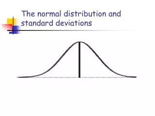
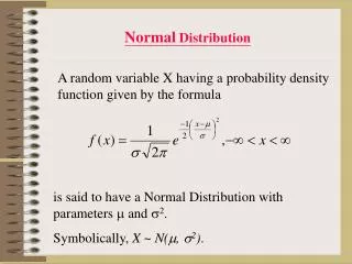
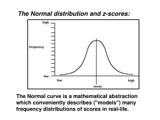
The Normal distribution and z-scores: The Normal curve is a mathematical abstraction which conveniently describes ("models") many frequency distributions of scores in real-life.
The area under the curve is directly proportional to the relative frequency of observations. e.g. here, 50% of scores fall below the mean, as does 50% of the area under the curve.
z-scores: z-scores are "standard scores". A z-score states the position of a raw score in relation to the mean of the distribution, using the standard deviation as the unit of measurement.
-3 -2 -1 0 +1 +2 +3 IQ (mean = 100, SD =15) as z-scores (mean = 0, SD = 1). z for 100 = (100-100) / 15 = 0, z for 115 = (115-100) / 15 = 1, z for 70 = (70-100) / 15 = -2, etc.
Why use z-scores? 1. z-scores make it easier to compare scores from distributions using different scales. e.g. two tests: Test A: Fred scores 78. Mean score = 70, SD = 8. Test B: Fred scores 78. Mean score = 66, SD = 6. Did Fred do better or worse on the second test?
Test A: as a z-score, z = (78-70) / 8 = 1.00 Test B: as a z-score , z = (78 - 66) / 6 = 2.00 Conclusion: Fred did much better on Test B.
2. z-scores enable us to determine the relationship between one score and the rest of the scores, using just one table for all normal distributions. e.g. If we have 480 scores, normally distributed with a mean of 60 and an SD of 8, how many would be 76 or above? (a) Graph the problem:
(b) Work out the z-score for 76: z = (X - X) / s = (76 - 60) / 8 = 16 / 8 = 2.00 (c) We need to know the size of the area beyond z (remember - the area under the Normal curve corresponds directly to the proportion of scores).
Many statistics books (and my website!) have z-score tables, giving us this information: (a) (b) * x 2 = 68% of scores + x 2 = 95% of scores # x 2 = 99.7% of scores (roughly!)
0.0228 (d) So: as a proportion of 1, 0.0228 of scores are likely to be 76 or more. As a percentage, = 2.28% As a number, 0.0228 * 480 = 10.94 scores.
How many scores would be 54 or less? Graph the problem: z = (X - X) / s = (54 - 60) / 8 = - 6 / 8 = - 0.75 Use table by ignoring the sign of z : “area beyond z” for 0.75 = 0.2266. Thus 22.7% of scores (109 scores) are 54 or less.
How many scores would be 76 or less? Subtract the area above 76, from the total area: 1.000 - 0.0228 = 0.9772 . Thus 97.72% of scores are 76 or less.
How many scores fall between the mean and 76? Use the “area between the mean and z” column in the table. For z = 2.00, the area is .4772. Thus 47.72% of scores lie between the mean and 76.
How many scores fall between 69 and 76? Find the area beyond 69; subtract from this the area beyond 76.
Find z for 69: = 1.125. “Area beyond z” = 0.1314. Find z for 76: = 2.00. “Area beyond z” = 0.0228. 0.1314 - 0.0228 = 0.1086 . Thus 10.86% of scores fall between 69 and 76 (52 out of 480).
? 89 92 Word comprehension test scores: Normal no. correct: mean = 92, SD = 6 out of 100 Brain-damaged person's no. correct: 89 out of 100. Is this person's comprehension significantly impaired? Step 1: graph the problem: Step 2: convert 89 into a z-score: z = (89 - 92) / 6 = - 3 / 6 = - 0.5
? 89 92 Step 3: use the table to find the "area beyond z" for our z of - 0.5: Area beyond z = 0.3085 Conclusion: .31 (31%) of normal people are likely to have a comprehension score this low or lower.
5% 200 ? Defining a "cut-off" point on a test (using a known area to find a raw score, instead of vice versa): We want to define "spider phobics" as those in the top 5% of scorers on our questionnaire. Mean = 200, SD = 50. What score cuts off the top 5%? Step 1: find the z-score that cuts off the top 5% ("Area beyond z = .05"). Step 2: convert to a raw score. X = mean + (z* SD). X = 200 + (1.64*50) = 282. Anyone scoring 282 or more is "phobic".
Hypothesis testing: • Step 1: • Scores often tend to be normally distributed. (b) Any given score can be expressed in terms of how much it differs from the mean of the population of scores to which it belongs (i.e., as a z-score).
population: mean = 500 g sample A: mean = 650g sample B: mean = 450g sample C: mean = 500g sample D: mean = 600g Brain size in hares: sample means and population means:
sample A mean sample H mean sample G mean sample F mean sample J mean sample B mean sample C mean sample D mean sample E mean sample K mean, etc..... The Central Limit Theorem in action: Frequency with which each sample mean occurs: the population mean, and the mean of the sample means
Population mean A particular sample mean Step 2: (a) Sample means tend to be normally distributed around the population mean (the "Central Limit Theorem"). (b) Any given sample mean can be expressed in terms of how much it differs from the population mean. (c) "Deviation from the mean" is the same as "probability of occurrence": a sample mean which is very deviant from the population mean is unlikely to occur.
Step 3: (a) Differences between the means of two samples from the same population are also normally distributed. Most samples from the same population should have similar means - hence most differences between sample means should be small. difference between mean of sample A and mean of sample B: high frequency of raw scores low mean of sample A mean of sample B low high sample means
(b) Any observed difference between two sample means could be due to either of two possibilities: 1. They are two samples from the same population, that happen to differ by chance (the "null hypothesis"); OR 2. They are not two samples from the same population, but instead come from two different populations (the "alternative hypothesis"). Convention: if the difference is so large that it will occur by chance only 5% of the time, believe it's "real" and not just due to chance.
Conclusions: The logic of z-scores underlies many statistical tests. 1. Scores are normally distributed around their mean. 2. Sample means are normally distributed around the population mean. 3. Differences between sample means are normally distributed around zero ("no difference"). We can exploit these phenomena in devising tests to help us decide whether or not an observed difference between sample means is due to chance.