Download
1 / 13
150 likes | 188 Views
A comprehensive overview of Linear Gaussian Models including Kalman Filter, Gaussian Mixtures, Hidden Markov Models, ICA, and more. Learn about properties of Gaussians, graphical models, and methods for learning and inference.

E N D
A Unifying Review of Linear Gaussian Models Summary Presentation 2/15/10 – Dae Il Kim Department of Computer Science Graduate Student Advisor: Erik Sudderth Ph.D.
Overview • Introduce the Basic Model • Discrete Time Linear Dynamical System (Kalman Filter) • Some nice properties of Gaussian distributions • Graphical Model: Static Model (Factor Analysis, PCA, SPCA) • Learning & Inference: Static Model • Graphical Model: Gaussian Mixture & Vector Quantization • Learning & Inference: GMMs & Quantization • Graphical Model: Discrete-State Dynamic Model (HMMs) • Independent Component Analysis • Conclusion
The Basic Model • Basic Model: Discrete Time Linear Dynamical System (Kalman Filter) Generative Model A = k x k state transition matrix C = p x k observation / generative matrix Additive Gaussian Noise Variations of this model produce: Factor Analysis Principal Component Analysis Mixtures of Gaussians Vector Quantization Independent Component Analysis Hidden Markov Models
Nice Properties of Gaussians • Conditional Independence • Markov Property • Inference in these models • Learning via Expectation Maximization (EM)
Graphical Model for Static Models Generative Model Additive Gaussian Noise Factor Analysis: Q = I & R is diagonal SPCA: Q = I & R = αI PCA: Q = I & R = lime0eI
Example of the generative process for PCA Bishop (2006) 2-dimensional observation space Marginal distribution for p(x) 1-dimensional latent space Z = latent variable X = observed variable
Learning & Inference: Static Models Analytically integrating over the joint, we obtain the marginal distribution of y. We can calculate our poterior using Bayes rule Our posterior now becomes another Gaussian Where beta is equal to: Note: Filtering and Smoothing reduce to the same problem in the static model since the time dependence is gone. We want to find P(x.|y.) over a single hidden state given the single observation. Inference can be performed simply by linear matrix projection and the result is also Gaussian.
Graphical Model: Gaussian Mixture Models & Vector Quantization Generative Model Additive Gaussian Noise (Winner Takes All - WTA)[x] = new vector with unity in the position of the largest coordinate of the input and zeros in all other positions. [0 0 1 ] Note: Each state x. is generated independently according to a fixed discrete probability histogram controlled by the mean and covariance of w. This model becomes a Vector Quantization model when:
Learning & Inference: GMMs & Quantization Computing the Likelihood for the data is straightforward Pi is the probability assigned by the Gaussian N(mu,Q) to the region of k-space in which the jth coordinate is larger than all the others. Calculating the posterior responsibility for each cluster is analagous to the E-Step in this model.
Gaussian Mixture Models Joint Distribution p(y,x) Marginal Distribution p(y) Pi is the probability assigned by the Gaussian N(mu,Q) to the region of k-space in which the jth coordinate is larger than all the others.
Graphical Model: Discrete-State Dynamic Models Generative Model Additive Gaussian Noise
Independent Component Analysis • ICA can be seen as a linear generative model with non-gaussian priors for the hidden variables or as a nonlinear generative model with gaussian priors for the hidden variables. Generative Model g(.) is a general nonlinearity that is invertible and differentiable The gradient learning rule to increase the likelihood:
Conclusion Many more potential models!