Download
1 / 11
110 likes | 136 Views
13. Monte Carlo II Scattering Codes. Rejection method Scattering albedo Plane parallel scattering atmosphere Optical depths & physical distances Emergent flux & intensity Internal intensity moments. P ( x ). P max. y 1. y 2. a. x 1. x 2. b. x. Rejection Method.

E N D
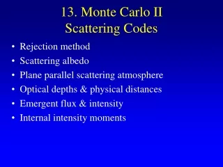
13. Monte Carlo IIScattering Codes • Rejection method • Scattering albedo • Plane parallel scattering atmosphere • Optical depths & physical distances • Emergent flux & intensity • Internal intensity moments
P(x) Pmax y1 y2 a x1 x2 b x Rejection Method The rejection method is used when we cannot invert the PDF as in the above examples to obtain analytic formulae for random q, l, etc. e.g., P(x) can be complicated function or tabulated Multiply two random numbers: uniform probability / area Choose x1 in range [a, b]: x1 = a + x(b - a), calculate P(x1) Choose y1 in range [0, Pmax]: y1 = xPmax If y1 > P(x1), reject x1. Choose new x2, y2 until y2 < P(x2): accept x2 Efficiency = Area under P(x)
Calculate p by the Rejection Method Choose N random positions (xi, yi): Choose xi in range [-R, R]: xi = (2x - 1) R Choose yi in range [-R, R]: yi = (2x - 1) R Reject (xi, yi) if xi2 + yi2 > R2 Number accepted / N = pR2 / 4R2 NA / N = p / 4 Increase accuracy (signal to noise) by increasing N. 2 R do i = 1, N x = 2.*ran – 1. y = 2.*ran –1. if ( (x*x + y*y) .lt. 1. ) NA = NA + 1 end do pi = 4.*NA / N FORTRAN 77:
Albedo When photon gets to interaction location at the randomly chosen optical depth, t, we must decide whether the photon is scattered or absorbed. We use the albedo or scattering probability. It is the ratio of scattering to total opacity: To decide if a photon is scattered we choose a random number in the range [0, 1] and scatter if x < a, otherwise the photon is absorbed. We now have the tools required to write a Monte Carlo radiation transfer program for isotropic scattering in a constant density slab…
Plane Parallel Code • Do loops, emitting photons, optical depths and physical distances, constant density slab • Intensity moments: mu-weighting, gridding, Lucy’s method of photon path-lengths for the mean intensity, Rybicki’s notes on path-length formulae for other moments • Output results for emergent intensity, intensity moments, comparison with Hopf function, boundary conditions! • 3D gridding, optical depth integration do-while loop, diffuse emission, web site with codes • Applications: RN, PNe, TTS, galaxies, planets, radiation pressure, atmospheric science • More complex grids, spherical logarithmic, trees, etc
Constant density slab of vertical optical depth tmax = nszmax. Normalized length units z = z / zmax. Emit photons Photon scatters in slab until: absorbed: terminate, start new photon z < 0: re-emit photon z > 1: escapes, “bin” photon Loop over photons Sample optical depths, test for absorption, test if photon is in slab
Emitting Photons: Photons need an initial starting location and direction. Isotropic emission from a surface.
Distance Traveled: Random optical depth t = -log x, and t = nsL, so distance traveled is: Scattering: Assume isotropic scattering, so new photon direction is: Absorb or Scatter: Scatter if x < a, otherwise the photon is absorbed, exit “do while in slab” loop and start a new photon.
Structure of FORTRAN 77 program: do i = 1, nphotons 1 call emit_photon do while ( (z .ge. 0.) .and. (z .le. 1.) ) ! photon is in slab L = -log(ran) * zmax / taumax z = z + L * nz ! update photon position, x,y,z if (ran .lt. albedo) then call scatter else goto 2 ! terminate photon end if end do if (z .le. 0.) goto 1 ! re-start photon bin photon according to direction 2 continue ! exit for absorbed photons, start a new photon end do
Intensity Moments The moments of the radiation field are (L5): We may compute these moments throughout the slab. First slit the slab into layers, then tally number of photons, weighted by powers of their direction cosines to obtain J, H, K. Contribution to specific intensity from a single photon is
Substitute these in the intensity moment equations and convert the integral to a summation to get: Note the mean flux, H, is just the net energy passing each level: number of photons traveling up minus number traveling down.