Download
1 / 23
230 likes | 310 Views
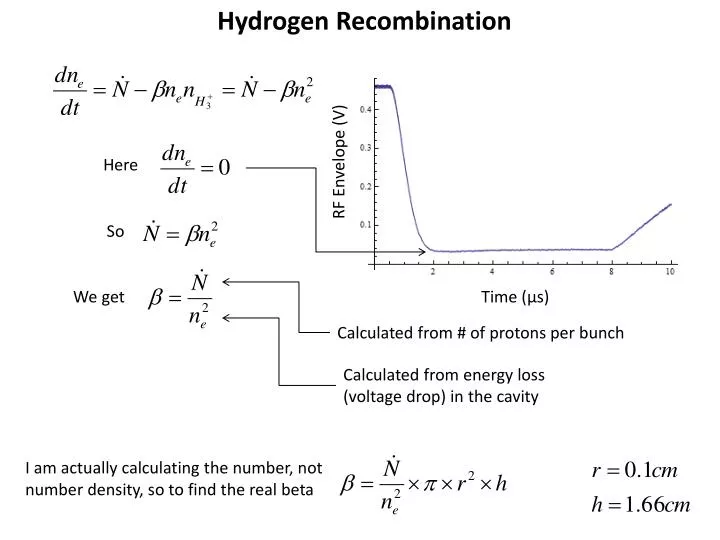
Hydrogen Recombination. RF Envelope (V). Here. So. We get. Time (µs). Calculated from # of protons per bunch. Calculated from energy loss (voltage drop) in the cavity. I am actually calculating the number, not number density, so to find the real beta. Model. V 0. RF Envelope (V). V.

E N D
Hydrogen Recombination RF Envelope (V) Here So We get Time (µs) Calculated from # of protons per bunch Calculated from energy loss (voltage drop) in the cavity I am actually calculating the number, not number density, so to find the real beta
Model V0 RF Envelope (V) V Time (µs)
Procedure Determine if RF pulse after was recorded (yes for >= July 25th) If yes, use RF pulse after to find cavity resistance, if no, use pulse during beam Read in pickup, downstream toroid, pickup pulse after (if it exists) Calculate cavity resistance Calculate beam intensity Determine parameters of interest (i.e. recombination rate)
Reading in the Data Pickup Signal Toroid Signal Average first 500 pts (100ns), then subtract from raw data Take absolute value of raw data Take a moving average over x data points, based on frequency, trying to sample over an integer number of cycles This is the envelope, and will be used for further analysis Average first 500 pts (100ns), then subtract from raw data Take absolute value of raw data Take a moving average over x data points to filter out background noise 424 points = good 422 points = better Pick 424 points
Determining Beam Intensity Find the average of the first 500 points (100 ns) from the toroid, this is the offset Find the minimum voltage after t=0 Subtract offset from minimum, that is the signal Calculate current = V / 50 Ohm * 10 turns Calculate charge = I * 7.5 µs Calculate # of protons per pulse = c / (1.6*10^-19 C/p) Calculate # of protons per bunch = #PpP / (7.5 µs * 200 MHz = 1500) V0 V
Determining Cavity Resistance Pick the maximum voltage after t=40 µs Select data from this point to the end Drop the first 5000 points (1µs) Fit remaining data with an exponential of the form τ = 1 / a3 (in units of µs) Rc = τ * 10-6 / C (capacitance of cavity) This is done, if possible, to the RF pulse after beam, as electrons are still present in the cavity when the klystron turns off L = 24.13 nH Typical values: 1.55 MΩ (pulse after) 1.66 MΩ (pulse during)
Determining the Voltage Drop in the Cavity Oscilloscope triggers on linac pulse Define the start of the beam to be when the toroid signal drops below 1 mV (this is pretty accurate – the noise is much less than this) The relative cable delay between toroid and pickup signals (48.07 ns) is taken into account Find this t0 in the pickup signal and the corresponding voltage Average over the previous 500 points (100 ns), call this the starting voltage, V0 Find the minimum voltage then average over 250 points (50 ns) on either side, call this the min voltage, V Remember, at this point V0 RF Envelope (V) V Time (µs)
Values That Are Calculated is the # of electrons per second, and is calculated from the # of protons per bunch, the ionization loss for protons in hydrogen, the gas pressure, and the bunch length (5 ns) is the # of electrons in the cavity, and is calculated from the power loss in the cavity , the energy loss per cycle per electron (dependent on the cavity voltage, pressure and frequency), and the RF frequency The temperature of the gas is also estimated, by Where in our case, the RMS KE of the swarm is approximated by Heylen as
30.1MV/m, model top 30MV/m, model top 20MV/m, model top 10MV/m, model top 10, 20 & 30.1 MV/m were all taken on 7/15, 30 MV/m was taken on 8/8
500psi, model top 950psi, model top 800psi, model top
Medium intensity, model top Low intensity, model top High intensity, 30.1MV/m, model top High intensity, model top 10, 20 & 30.1 MV/m were all taken on 7/15, 30 MV/m was taken on 8/8
30MV/m, model bottom 30.1MV/m, model bottom 20MV/m, model bottom 10MV/m, model bottom 10, 20 & 30.1 MV/m were all taken on 7/15, 30 MV/m was taken on 8/8
800psi, model bottom 950psi, model bottom 500psi, model bottom
High, model bottom 30.1MV/m, High, model bottom Low, model bottom Medium, model bottom 10, 20 & 30.1 MV/m were all taken on 7/15, 30 MV/m was taken on 8/8
10MV/m, model top 20MV/m, model top 30MV/m, model top 30.1MV/m, model top 10, 20 & 30.1 MV/m were all taken on 7/15, 30 MV/m was taken on 8/8
950psi, model top 800psi, model top 500psi, model top
Medium intensity, model top High intensity, model top Low intensity, model top 30.1MV/m, high intensity, model top 10, 20 & 30.1 MV/m were all taken on 7/15, 30 MV/m was taken on 8/8
30.1MV/m 30MV/m 20MV/m 10MV/m 10, 20 & 30.1 MV/m were all taken on 7/15, 30 MV/m was taken on 8/8
500psi 800psi 950psi
Medium intensity Low intensity 30.1MV/m, high intensity High intensity 10, 20 & 30.1 MV/m were all taken on 7/15, 30 MV/m was taken on 8/8