Download
1 / 18
190 likes | 293 Views
Circuits II EE221 Optimization of Filter Parameters Instructor: Kevin D. Donohue. Iteration, Objective/Error Functions, Visualization. Matlab and Parameter Optimization:.

E N D
Circuits IIEE221Optimization of Filter ParametersInstructor: Kevin D. Donohue Iteration, Objective/Error Functions, Visualization
Matlab and Parameter Optimization: • If equations can be developed to relate design parameters to the error/objective criteria, and they can be solved directly, the problem is finished. Unfortunately in many cases, the large number of parameters or the nonlinear relationship between them, makes a direct (closed-form) solution difficult or impossible. • The performance equations can, however, be examined through programs, such as Matlab, and optimization performed with a creative strategy for iterating through guesses of critical parameters until error reaches a practical minimum. • Matlab functions: Available Matlab functions can be combined together to create your own function useful for your optimization task. • Example: Create a Matlab function that evaluates transfer function samples of a first-order low-pass filter over an array of frequency axis points (in Hz), for a given cutoff frequency (in Hz), and the gain at DC (in dB).
Function for Use in Iteration Process • 1) Use a text editor to create a file lpf1.m (Matlab program files always end in .m). • 2) Then enter the following text. • function h = lpf1(f,fc,gdb) • % This function evaluates complex points of a first • % order low-pass filter with cut-off frequency fc • % in Hertz, and a gain in dB at DC of gdb. The • % function syntax is: • % • % tflp = lpf1(f, fc, gdb) • % • % where f is an array of points in Hertz where the • % function is eavluated at, and tfpl is the array of • % complex evaluation points. • s = j*2*pi*f; % compute complex frequencies along j omega axis. • gdc = 10^(gdb/20); % convert gain in dB to linear gain. • h = gdc./(s/(2*pi*fc) + 1 ); % Evaluate TF point by point • 3) Save the file in your “working directory” and execute in Matlab just like any other function. If you type help lpf1 in Matlab, the first sequence of comments will print to the screen.
Function for Use in Iteration Process 4) All variables defined inside the function will be undefined when the function is through (local variables).Create an analogous function for a high-pass filter: 1) Create file with a text editor called hpf1.m and enter: function h = hpf1(f,fc,gdb) % This function evaluates complex points of a first % order high-pass filter with cut-off frequency fc % in Hertz, and a gain in dB at infinity of gdb. % The function syntax is: % % tfhp = hpf1(f, fc, gdb) % % where f is an array of points in Hertz where the % function is evaluated at, and tfhp is the array of % complex evaluation points. % s = j*2*pi*f; % compute complex frequencies along j omega axis. ginf=10^(gdb/20); % convert gain in dB to linear gain. • h = ginf*(s/(2*pi*fc))./(s/(2*pi*fc) + 1 ); % Evaluate TF point by point
Script for Optimization Matlab Scripts: Matlab functions can be combined together to create a series of commands to be executed. Example: Create a Matlab script to examine the mean and variance error between a cascaded low-pass and high-pass filter, and a band-pass-like transfer function specification consisting of a flat 10 dB passband extending from 5 kHz to 50 kHz with a 20 dB per decade roll-off at either end of the passband. The gain in the passband is 10 dB. Only consider the error from 500 Hz to 500 kHz. • Strategy: Since the major portion of overlap between the passbands of the LPF and HPF will exist between the cut-off frequencies, set the gains equal to about 5.6 dB each (should put the combined gain close to 10db). Now consider minimizing error with respect to the cut-off frequencies of the LPF and the HPF. The gain can be adjusted later if assumption on the passband gain is not accurate. 2) Create a file in a text editor called ex6.m, and enter: f =logspace(log10(500),log10(500e3), 512); % define axis for evaluation % Create target function (Described in Example) ht = zeros(1,512); % Set up array to fill with function points
Script for Optimization % Loop through each linear section piece-wise, to create target shape for k=1:512 % For points less than 5kHz create a line on a log scale if( f(k) < 5e3) , ht(k) = -10 + 20*log10(f(k)/500); % For points greater than 5kHz and less than 50kHz elseif(f(k) < 5e4), ht(k) = 10; % for points greater than 50kHz create a line on a % log scale else ht(k) = 10 - 20*log10(f(k)/5e4); end end % Note the above code has nothing to do with your project % It should not be seen in any of your codes figure(1) semilogx(f,ht) % Check to see if it did what we wanted it to grid title('Target TF') xlabel('Hertz') ylabel('dB') pause % Script will pause until the keyboard is struck % Set up nested loops to vary the cutoff frequencies for HPF and LPF % Try a neighborhood of frequencies around f= 5 kHz and 50 kHz. fhc = linspace(3500,7500,25); % Select a set of high-pass cut-offs flc = linspace(35000, 55000, 25); % Select a set of low-pass cut-offs
Script for Optimization % Set up arrays to store computed error terms em = zeros(25,25); % mean error (bias) ev = zeros(25,25); % variance error (consistency of fit) % Fix Gain at 5.6 dB => 10^(5.6/20) = 1.9055 and optimize for low-pass % and high-pass cutoff % Note, this may not be the best gain, but is just an initial guess. for k=1:25, for n=1:25, h = lpf1(f,flc(k),5.6).*hpf1(f,fhc(n),5.6); % Compute Resultant TF % Compute errors em(k,n) = mean(ht-20*log10(abs(h))); ev(k,n) = std(ht-20*log10(abs(h))); %This is actually square root of the % variance, which is just as good in terms of finding a minimum point. end end [k,n] = find(abs(em) == min(min(abs(em))))%find mean error index close to 0 % look at optimal TF h = lpf1(f,flc(k),5.6).*hpf1(f,fhc(n),5.6); % Compute Resultant TF % points at optimum semilogx(f,20*log10(abs(h)),'g') hold on semilogx(f, ht,':r') hold off title('Compare target with design TF for minimum mean error') xlabel('Hertz')
Script for Optimization % To get a better view, try an intensity plot of the same data: figure(3) % Plot Mean Error imagesc(fhc, flc, abs(em)) colormap('gray') colorbar title('mean error') xlabel(' High-pass cut-off') ylabel(' Low-pass cut-off') figure(4) % Plot Variance (standard deviation) Error imagesc(fhc, flc, ev) colormap('gray') colorbar xlabel(' High-pass cut-off') ylabel(' Low-pass cut-off') title('standard deviation error') pause 3) Save file and type ex6 at Matlab prompt. These commands will execute and when finished, all variables defined in the script will still be available in the Matlab workspace.
Script for Optimization ylabel('dB') flcmm = flc(k) % Convert index to frequency value fhcmm = fhc(n) % Convert index to frequency value pause [k,n] = find(ev == min(min(ev))) % find index of minimum variance error • % Compute Resultant TF points at optimum h = lpf1(f,flc(k),5.6).*hpf1(f,fhc(n),5.6) figure(2) semilogx(f,20*log10(abs(h)),'g') hold on semilogx(f, ht,':r') hold off title('Compare target with design TF for minimum variance error') xlabel('Hertz') ylabel('dB') flcsd = flc(k) % Convert index to frequency value fhcsd = fhc(n) % Convert index to frequency value pause figure(3) mesh(fhc, flc, abs(em)) % Look at graphic distribution of error. title('mean error') figure(4) mesh(fhc, flc, ev) title('standard deviation error') pause
Script for Optimization • % Changing the color map to something other than gray may help in • % observing changes in levels. Use the 'jet' color scheme To get a • % better view, try an intensity plot of the same data: • figure(5) • imagesc(fhc, flc, abs(em)) • colormap('jet') • colorbar • title('mean error') • xlabel(' High-pass cut-off') • ylabel(' Low-pass cut-off') • figure(6) • imagesc(fhc, flc, ev) • colormap('jet') • colorbar • xlabel(' High-pass cut-off') • ylabel(' Low-pass cut-off') • title('standard deviation error') 3) Save file and type ex6 at Matlab prompt. These commands will execute. When finished, all variables defined in the script will still be available in the Matlab workspace.
Optimization Results • 4) The results of this program should yield a variance error at k=3 and n=16, which corresponds to cutoffs at 6000 Hz and 41667 Hz. Further improvement can be obtained by fixing the cutoffs and varying the gain. The following is the output of the previous script: • Mean Error • k = • 12 • n = • 8 • flcmm = • 4.4167e+004 • fhcmm = • 4.6667e+003 • Variance Error • k = • 9 • n = • 16 • flcsd = • 4.1667e+004 • fhcsd = • 6000
Optimization Iterated Error Surfaces (Intensity Image) Result for color map ‘gray’
Optimization Iterated Error Surfaces (Intensity Image) Result for color map ‘jet’
Parameter Optimization BPF Example: • Example: Create a Matlab script that evaluates matching a desired transfer function shape by adding 3 second-order band-pass filters and varies the mid frequency bandwidth to variance error. The test points are at 100, 500, 1000, 2000, 3000, and 5000 Hz and correspond to TF magnitudes of 0, 6, 10, 2, 6, and -1 dB. • See script opt1.m on course web site • http://www.engr.uky.edu/~donohue/ee221/mfile.html • Since shape is the criterion, only need to evaluate variance error:>> errv(k) = std(ht-tfg)^2; % Compute error for this bandwidth where ht is the vector of test point magnitudes for the target TF and tgf is the vector of corresponding points evaluated on the kth synthesized filter
Parameter Optimization BPF Example: • Target TF and Initial Guess • % Initial guess for parameters of 3 BPFs in parallel • % BPF1 • f01 = 1000; % Center Frequency Hz • b1 = 600; % Bandwidth Hz • g1 = 10; % Gain at center frequency in dB • % BPF2 • f02 = 3000; % Center Frequency Hz • b2 = 2000; % Bandwidth Hz • g2 = 6; % Gain at center frequency in dB • % BPF3 • % The third BPF helps fit the shape at the low end • % to slow down the roll off from the middle BPF • f03 = 300; % Center Frequency Hz • b3 = 500; % Bandwidth Hz • g3 = 4; % Gain at center frequency in dB
Parameter Optimization BPF Example: • With all other parameters fixed, vary bandwidth of middle BPF (BPF1) from 200 to 2000 Hz in linear steps of 10. Various iterations:
Parameter Optimization BPF Example • Iteration corresponding to minimum variance error.


![[f´‚nE˘RIks]](https://cdn0.slideserve.com/1072532/f-ne-riks-dt.jpg)