Download
1 / 24
240 likes | 412 Views
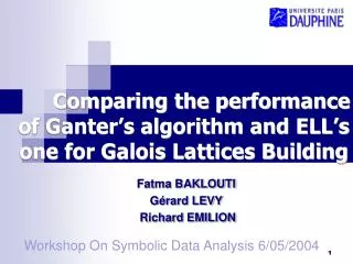
Comparing the performance of Ganter’s algorithm and ELL’s one for Galois Lattices Building. Fatma BAKLOUTI Gérard LEVY Richard EMILION. Workshop On Symbolic Data Analysis 6/05/2004. Plan. Galois Lattices Two algorithms : Ganter ELL Experimental performance analysis

E N D
Comparing the performance of Ganter’s algorithm and ELL’s one for Galois Lattices Building Fatma BAKLOUTI Gérard LEVY Richard EMILION Workshop On Symbolic Data Analysis 6/05/2004
Plan • Galois Lattices • Two algorithms : • Ganter • ELL • Experimental performance analysis • Conclusion and perspectives
Galois Lattices • Using Galois Lattice (mathematical structure) for solving Data Mining problems. • References : • Birkhoff’s Lattice Theory: 1940, 1973 • Barbut & Monjardet : 1970 • Wille : 1982 • Chein, Norris, Ganter, Bordat, … • Diday, Duquenne, … • Emilion, Lévy, Diday, Lambert • Basic Concepts : Context, Galois connection, Concept.
Galois Lattices - Definition • Context = (O, A, I) : • O : finite set of examples • A : finite set of attributes • I : binary relation between O and A, (I O x A) • Example : O
Galois Lattices - Definition • Galois connection • Oi O and Ai A, we define f et g like this : • f : P(O) P(A) f(Oi) = {a A / (o,a) I, o Oi} intent • g: P(A) P(O) g(Ai) = {o O / (o,a) I, a Ai} extent • f et g are decreasingapplications • h =g · f and k = f · g, are : • Increasing O1 O2 h (O1) h (O2) • Extensive O1 h (O1) • Idempotent h (O1) = h · h (O1) • h and k are closure operators. • (f,g) = Galois connection between P(O) and P(A)
Galois Lattices - Definition • Concept • Oi O et Ai A, • (Oi, Ai) is a concept iff Oi is the extent of AiandAi is the intentof Oi • Oi = g (Ai) and Ai = f(Oi) • L ={(Oi, Ai) P(O)P(A) / Oi= g(Ai) et Ai = f(Oi)} : concepts set. • L: ordered set by the relationship ≤ • (O1, A1) ≤ (O2, A2) iff O1 O2 (or A2 A1). • Galois Lattice • T=(L, ≤) an ordered set of concepts.
Galois Lattices - Definition • Concept: Example • O1 = {6,7} f(O1)= {a,c} intent • A1 = {a,c} g(A1)= {1,2,3,4,6,7}extent • Remark: h(O1)= g · f(O1)= g(A1) ≠ O1 • ({6,7} , {a,c}) L • ({1,2,3,4,6,7}, {a,c}) L Because: h({1,2,3,4,6,7}) = g · f({1,2,3,4,6,7}) = g ({a,c}) = {1,2,3,4,6,7}
1234567, a 123467, ac 123456, ab 12345, abd 12346, abc 12356, abe 1247, acf 1234, abcd 1235, abde 1236, abce 124, abcdf 135, abdeg 123, abcde 236, abceh 12, abcdef 13, abcdeg 23, abcdeh 1, abcdefg 2, abcdefh 3, abcdegh Ø, abcdefgh
Lexicographicorder 1111 0000 0001 0010 0011 0111 1000 a a+ a* x1 a ( 0 1 1 1 ) 0 1 a+ ( 1 0 0 0 ) 0 0 1 1 x2 1 1 0 1 0 1 a* ( 1 1 1 1 ) 0 0 x3 0 1 0 1 0 1 1 0 1 1 1 0 0 x4 Ganter Algorithm a (a1, …, ai-1, ai, bi+1, …, bn) a+ (a1, …, ai-1, 1+ai, 0, …, 0 ) a* (a1, …, ai-1, bi, bi+1,…, bn) k (a+) = f (g (a+)) = y If a+ y a* y closestclosed ofa a = a*
a ( 1, 1, 5, 2, 1 ) 0 x5 1 0 x4 2 0 x3 5 0 x2 3 0 x1 3 Ganter Algorithm a (a1, …, ai-1, ai, bi+1, …, bn) a+ (a1, …, ai-1, 1+ai,0, … ,0 ) a* (a1, …, ai-1, bi, bi+1,…, bn) Example : a+( 1, 2, 0, 0, 0 ) a*( 1, 3, 5, 2, 1 ) k (a+) = f (g (a+)) = ?
Generalized Galois Lattices • Context : < I, F, d > • T = <F, , , ≤> • Tj= <Fj, j, j, ≤j> for all j de J, J = [1,n] • d: I F • di = (di1,…, dij,…, din) :description of the individual i relatively to the attributes j of J. 1 2 j n 1 i k • x I • f (x) = d(i) i x Intent • z F • g (z) = { i I | z ≤ d(i) } Extent Individuals I
ELL Algorithm • Let X0 and K Ø and i0 K. 1) h (X0 U {i0}) = { i I : f (X0) f (i0) ≤ f (i) } = X0 U A (X0 h (X0) h (X0U {i0}) ) where A = { i I \ X0: f (X0) f (i0) ≤ f (i) } • For two disjoint subsets X0 and K of I, ELL lists all the closed sets of I obtained by extending X0 with some elements of K. 2) If a closed set contains X0 and i0, then it also contains A. Hence, if A K then (X0 U A) is the smallest closed set containing X0and i0 and contained within X0 U K. X = X0U A, K = K / A 3) If a closed set contains X0 and does not contain i0, then it also does not contain any element of the set. R = { i K: f (X0) f (i) ≤ f (i0) }, K = K / R
ELL Algorithm GL = Ø. Procedure:Closed (X0, K) Var i0: element of I, z, z0: elements of F; X, A, R: subsets of I; begin z0 = f (X0); if K ≠ Ø then begin choose an element i 0 of K; z = z0 f (i0); A = {i I \ X0: z ≤ f (i)}; if A K then begin X = X0 U A; insert node (X, z) in ELL; Closed (X, K\A); end; R = {i K: z0 f (i) ≤ f (i0)}; Closed (X0, K \ R); end; end;
Example • X0 = Ø and K = I = {1, 2, 3, 4, 5} • We choose the element i0 = 1 of K; • f (X0) = z = 1F = (3, 2, 3) • z = z0 f (i0) = (3, 2, 3) (0, 1, 1) = (0, 1, 1) • h (X) = { i I : f (X0) f (i0) ≤ f (i) } = {1, 4} • A = { i I \ X0: z ≤ f (i)}= {1, 4} • A K • X = {1, 4} and z = (0, 1, 1), (X, z) Closed item pair • X = X0 A = Ø {1, 4} • X0 = {1, 4} and K = {2, 3, 5} • We choose the element i0 = 2 of K; • f (X0) = z = (0, 1, 1) • z = z0 f (i0) = (0, 1, 1) (2, 0, 1) = (0, 0, 1) • A = {i I - X0: z ≤ f (i)}= {2, 3} K • X = X0 A = {1, 4, 2, 3} • X = {1, 4, 2, 3} and z = (0, 0, 1), (X, z) Closed item pair • ….
Total number of closed pairs (X, z) of lattice T =GL (C) =14. • pair (1)= x = {1,4,} z = {0,1,1,} • pair (2)= x = {1,4,3,2,} z = {0,0,1,} • pair (3)= x = {1,4,3,2,5,} z = {0,0,0,} • pair (4)= x = {1,4,5,} z = {0,1,0,} • pair (5)= x = {2,3,} z = {2,0,1,} • pair (6)= x = {2,3,5,} z = {2,0,0,} • pair (7)= x = {2,3,5,4,} z = {1,0,0,} • pair (8)= x = {2,3,4,} z = {1,0,1,} • pair (9)= x = {5,} z = {2,1,0,} • pair (10)= x = {5,4,} z = {1,1,0,} • pair (11)= x = {3,} z = {3,0,3,} • pair (12)= x = {3,4,} z = {1,0,3,} • pair (13)= x = {4,} z = {1,2,3,} • pair (14)= x = {} z = {3,2,3,} • The case X0 = Ø isn’t treated by the algorithm so the test must be added. • In this example: • X = Ø • f (X) = z = 1F = (3, 2, 3) • g (z) = {i I/ z ≤ d (i)} = Ø • X = Ø and z = 1F = (3, 2, 3), (X, z): Closed item pair
Experimental Performance Analysis • Time in ms M: number of individuals • CN : Closed Number N : number of attributes
Other Data types … b1 [0,1] [0,4] Intent: f (x) = d(i) i x x = {1,3} x1 x3 = [1,1] [1,3] = [1,1] y1 y3 = [3,4] [0,4] = [3,4] Extent : g (z) = {i I | z d(i)} z = [1,1] [3,4] g (z) = {1,3}
1 ; ([0,1] [0,4]) 7 10 8 {3}; ([1,1] [0,4]) {4} ; ([0,1] [0,2]) {5} ; ([0,0] [3,3]) 2 9 {1,3} ; ([1,1] [3,4]) {4,5} ; ([0,0] ) 5 6 {1,3,5} ; ( [3,3]) {2,3,4} ; ([1,1] [0,2]) 3 {1,2,3,4} ; ([1,1] ) 4 {1,2,3,4,5} ; ( )
Conclusion and perspectives Problems • Large data volume: Partition data on different server nodes Process in parallel locally Group results on one (client) node Post-process Our tool: SDDS(Scalable Distributed Data Structures )
Conclusion and perspectives Solutions • Column-sharing • Row-sharing «ParallelAlgorithms for General Galois lattices building» Fatma BAKLOUTI and Gérard LEVY 4th Int. Workshop on Distributed Structures (WDAS 2003)
Conclusion and perspectives • Generalized Galois Lattices. • Problem of large data base can be perhaps resolved in our way. • Sharing context into two subsets. • Possibility of building different architectures for station’s networks.