Download
1 / 19
190 likes | 204 Views
This presentation discusses the phase diagram of the Gross-Witten-Wadia (GWW) phase transition in matrix quantum mechanics with a chemical potential. The thermodynamic aspects of quantum gravity in AdS spacetime, the model, and the results of both the bosonic and fermionic models are explored. The talk also covers the rational hybrid Monte Carlo (RHMC) simulation used and the computational techniques employed to solve the problem efficiently.

E N D
"Phase diagram of the GWW phase transition of thematrix quantum mechanics with a chemical potential" Takehiro Azuma (Setsunan Univ.) From Strings to LHC IV, Sinclairs Retreat, Chalsa Mar. 10th 2017, 14:25-14:50 with Pallab Basu (ICTS,TIFR) and Prasant Samantray (IIT, Indore)
1. Introduction Thermodynamic aspects of quantum gravity in AdS spacetime: ・Small blackhole (SBH): Unstable. Horizon radius smaller than AdS ・Big blackhole (BBH): Stable. Horizon radius comparable to AdS Gross-Witten-Wadia (GWW) phase transition of the gauge theory and the blackhole phase transition [L. Alvarez-Gaume, C. Gomez, H. Liu and S.R. Wadia, hep-th/0502227]
2. The model Finite-temperaturematrix quantum mechanics with a chemical potential S = Sb + Sf + Sg, where(μ=1,2,….D, β=1/T) ・Bosonic (S=Sb+Sg): D is an arbitrary integer D=2,3,… ・Fermionic(S=Sb+Sf+Sg): (D,p)=(3,2),(5,4),(9,16) (For D=9, the fermion is Majorana-Weyl ( Ψ→Ψ ) In the following,we focus on D=3.)
2. The model A(t), Xμ(t), Ψ(t) : N×N Hermitian matrix Boundary conditions: Static diagonal gauge: ⇒ Add the gauge-fixing term Underthisgauge Supersymmetry for S=Sb+Sf(μ=0), broken at μ≠0.
2. The model Previous works for μ=0 (without Sg) SUSY (S=Sb+Sf) Bosonic (S=Sb) de-confinement <|u1|> <|u1|> confinement T T [Quoted for D=9 from N. Kawahara, J. Nishimura and S. Takeuchi, arXiv:0706.3517] [Quoted for D=9 from K.N. Anagnostopoulos, M. Hanada, J. Nishimura and S. Takeuchi, arXiv:0707.4454] Confinement-deconfinement phase transition at T=Tc0 Absence of phase transition <|u1|>= a0exp(-a1/T)
3. Result of the bosonic model Bosonic model without fermion S=Sb+Sg [T. Azuma, P. Basu and S.R. Wadia, arXiv:0710.5873] ResultofD=3(D=2,6,9cases are similar) ρ(θ) <|u1|> D=3,N=48 <|u2|> D=3,N=48 D=3,N=48 Around (μc,Tc)=(0.2,0.7), Critical points (μc, Tc) at <|u1|>=1/2 develops a gap. At (μc, Tc), d<|u1,2|>/dμand d<|u1,2|>/dTare not smooth (d2<|u1,2|>/dμ2 and d2<|u1,2|>/dT2 are discontinuous) ⇒ suggests third-order phase transition.
3. Result of the bosonic model D=3,N=48 D=3,N=48 <|u1|> D=3,N=48 D=3,N=48 <|u2|>
3. Result of the bosonic model <|u1|> D=3,N=48 D=3,N=48 D=3,N=48 <|u2|> D=3,N=48
3. Result of the bosonic model When μ=0, at the critical point Tc0=1.1, there is a first-order phase transition at small D. [T. Azuma, T. Morita and S. Takeuchi, arXiv:1403.7764] We fit the susceptibility with (γ,p,c) as p=1 ⇒ suggests first-order phase transition. [M. Fukugita, H. Mino, M. Okawa and A. Ukawa, Phys. Rev. Lett.65, 816 (1990)] D=3 first-order not first-order
4. Result of the fermionic model The model with fermion (D=3) S=Sb+Sf+Sg Γμ=σ μ (μ=1,2,3) Non-lattice simulation with Fourier expansion [K.N. Anagnostopoulos, M. Hanada, J. Nishimura and S. Takeuchi, arXiv:0707.4454] Integrating out Ψ ⇒ N0×N0 matrix (N0 = 2×2Λ×(N2-1) ) traceless adjoint r=-Λ+1/2,…Λ-1/2 Gamma matrix [4(D=5), 16(D=9)] D=3: is real ⇒ no sign problem.
4. Result of the fermionic model ResultofD=3, N=16, after large-Λ extrapolation: <|u1|> <|u1|> Gapped⇔ Ungapped Possible phase transitions at (μc,Tc) where <|u1|>=0.5. large-Λ extrapolation <|u1|> Λ=8
4. Result of the fermionic model ResultofD=3, N=16, after large-Λ extrapolation: History of at Λ=3 No instability in the typical (μ,T) region.
4. Result of the fermionic model Phase diagram for D=2,3,6,9 (boson) and D=3(fermion). Some phase transitions at(μc ,Tc) where <|u1|>=0.5 D=3 SUSY, μ=0: <|u1|>= a0 exp(-a1/T) a0=1.03(1), a1=0.19(1) ⇒<|u1|>=0.5 at T=0.28. [M. Hanada, S. Matsuura, J. Nishimura and D. Robles-Llana, arXiv:1012.2913] μ=0: <|u1|>= 0.5 at Tc=1.39×0.52.30≃0.28 Fittingofthecriticalpointby Tc=a(0.5-μc)b.
5. Summary We have studied the matrix quantum mechanics with a chemical potential ・bosonic model ⇒ GWW-type third-order phase transition (except for very small μ) ・phase diagram of the bosonic/fermionic model
backup: GWW phase transition [D.J. Gross and E. Witten, Phys. Rev. D21 (1980) 446, S.R. Wadia, Phys. Lett. B93 (1980) 403] Gross-Witten-Wadia (GWW)type third-order phase transition
backup: GWW phase transition Continuous at μ=1/2. Discontinuous at μ=1/2. ⇒For free energy, d3F/dμ3 is discontinuous.
backup: RHMC Simulation via Rational Hybrid Monte Carlo (RHMC) algorithm. [Chap 6,7 of B.Ydri, arXiv:1506.02567,for a review] We exploit the rational approximation after a proper rescaling. (typically Q=15⇒valid at 10-12c<x<c) ak, bk come from Remez algorithm. [M. A. Clark and A. D. Kennedy, https://github.com/mikeaclark/AlgRemez] F: bosonic N0-dim vector (called pseudofermion)
backup: RHMC Hot spot (most time-consuming part) of RHMC: ⇒Solving by conjugate gradient (CG) method. Multiplication ⇒ is a very sparse matrix. No need to build explicitly. ⇒CPU cost is O(N3)per CG iteration The required CG iteration time depends on T. (while direct calculation of -1 costs O(N6).) Multimass CG solver: Solve only for the smallest bk ⇒The rest can be obtained as a byproduct, which saves O(Q) CPU cost. [B. Jegerlehner, hep-lat/9612014 ] 18
backup: RHMC Conjugate Gradient (CG) method Iterative algorithm to solve the linear equation Ax=b (A: symmetric, positive-definite n×n matrix) Initial config. (for brevity, no preconditioning on x0 here) Iterate this until The approximate answer of Ax=b is x=xk+1.