Vector Space Classfication
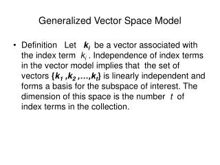
Vector Space Classfication. Chapter 11. Chapter Index. 14.1 Introduction 14.2 Rocchio Classification 14.3 k Nearest Neighbor Classification 14.4 Linear vs. Nonlinear Classifiers 14.5 두 가지 이상의 클래스에서의 분류법 14.6 The bias-variance tradeoff. Introduction.

Vector Space Classfication
E N D
Presentation Transcript
Vector Space Classfication Chapter 11
Chapter Index • 14.1 Introduction • 14.2 Rocchio Classification • 14.3 k Nearest NeighborClassification • 14.4 Linearvs. Nonlinear Classifiers • 14.5 두 가지 이상의 클래스에서의 분류법 • 14.6 The bias-variance tradeoff
Introduction • 이번 Chapter에서는 chapter6에서 다뤘던 vector space model을 이용하여 문서를 분류하는 방법을 사용한다. Vector space model에서의 분류는 contiguity hypothesis에 기반하고 있다. • Contiguity hypothesis • 같은 클래스의 문서는 연속적인 영역을 이루고 있으며, 클래스끼리 겹치지 않는다. • 이번 Chapter에서는 2가지의 분류 기법을 소개한다. • Rocchio 분류법은 centroid 혹은 prototype이 중심이 된 영역으로 vector space를 분리한다. • 간단하고 효율적이지만, 문서들이 원 모양(spherical)으로 분포하지 않으면 결과가 좋지 않다. • kNN분류법은 보통 학습을 거쳐 사용하지만 학습을 거치지 않고서도 사용이 가능하다. • 덜 효율적이지만문서들이 원 모양으로 분포하지 않아도 결과를 잘 내고, training set이 큰 경우 Rocchio 분류법보다 복잡한 분류를 더 잘 수행한다.
Rocchio Classification • China, UK, Kenya로 문서를 나누고 있다. • 나누는 경계를 decision boundary라고 부른다. • Star 문서를 새로 분류하고자 할 때, 그림에서 문서는 China의 영역에 있으므로 이 문서를 China로 분류한다. • Rocchio 분류의 적용법 • 각 클래스의 문서 vector의 centroid를 찾는다. • 새로운 문서 분류 시 가장 가까운 centroid의 클래스로 분류한다. • Rocchio 분류에서는 centroid를 사용하여 경계를 결정한다. • 한 클래스의 Centroid c는 클래스 멤버들의 벡터의 평균으로 나타난다. • Dc : 문서집합D에서 클래스가 c인 문서들 • v(d) : d 문서의 normalized vector • Centroid vector는 unit vector가 아닐 수도 있다.
Rocchio Classification • 클래스의 boundary는 각 centroid에서 같은 거리에 있는 점들이 선을 형성하게 된다. • 그림에서 |a1|=|a2|, |b1|=|b2|, |c1|=|c2|등을 만족하는 선 • Boundary는 다음을 만족하는 point x의 집합이다. • w는 M차원의 normal vector이고 b는 상수이다. • 2차원에서는 w1x1 + w2x2 = b 의 형태로, • 3차원에서는 w1x1 + w2x2 + w3x3 = b 의 형태로 나타난다. • 위 직선(혹은 평면)은 hyperspace를 둘로 나누게 된다. • Hyperplane을 분할하는 vector w와 boundary b는 다음과 같이 구할 수 있다. ( ※ c1, c2는 norm vector의 평균 ) decision hyperplane u(c2) u(c1) (0,1)-(1,2) →
Rocchio Classification • 예제 14.1) 2개의 centroid • μc = 1/3*(d1+d2+d3) • μc’ = 1*(d4) • 문서 d5를 분류하는 과정 • |μc – d5| ≒ 1.15 • |μc‘ – d5| ≒ 0.0 • Rocciho assigns d5 to μc‘ • Hyperplane을 분할하는 parameter들은 다음과 같다. • w =μc- μc’ ≒ ( 0, -0.71, -0.71, 0.33, 0.33, 0.33 )T • b = 0.5 * ( |μc|2 - |μc’|2 ) = 0.5 * ( 0.571577^2 - 1.00409^2 ) = -0.340748 ≒ -1/3 • Hyperplane에 속하는지 분류된 문서를 확인해 보기 • W · d1 = 0*0 + -0.71*0 + -0.71*0 + 1/3*0 + 1/3*1 + 1/3*0 ≒1/3 > b • d2, d3도 위와 같은 계산으로 ≒ 1/3 ≥ b • w · d4 = -1 < b • 클래스 c 는 hyperplane 위에 있고, c’ 는 hyperplane 밑에 있는 것을 확인할 수 있음
Rocchio Classification • 9장에서 다뤘던 Rocchio relevance feedback은 Rocchio classification의 응용 • Relevance feedback method는 2클래스의 분류를 위한 것 – Relevant / non-relevant • Rocchio 분류법은 multimodal 클래스 분류에 약하다. • “a” 문서들은 2 클러스터를 이루고 있다. • 따라서 A클러스터의 centroid는 정확히 정의될 수 없다. • 새로운 O 문서는 성격이 “b” 문서들에 가까우나, A클래스의 Centeroid에 더 가깝기 때문에 A클래스로 분류된다. • Multimodal class의 예: Burma로 이름이 바뀐 Myanmar • 보통 2-클래스 classifier은 china와 같이 한 부분의 영역을 차지 하는 클래스와 전체적으로 산개되어 있는 negative 문서들을 구분한다. 원 모양 반경 안에 균일하게 문서가 분포하고 있는 경우는 실제로는 드문 경우이므로 다음과 같이 boundary에 대한 decision rule에 negative 문서를 반영한다. →
Rocchio Classification • Rocchio classification의 time complexity는 다음과 같다. • Training • θ(|D|Lave + |C||V|) • Lave : 문서 안의 평균 단어 수 • D: collection의 문서 개수 • C: 클래스의 개수 • V: collection의 단어 개수 • Testing • θ(|C|Ma) • C: 클래스의 개수 • Ma: 문서 안의 unique한 단어 개수
k Nearest Neighbor Classification • kNN = k Nearest Neighbor • 클래스 c인 문서 d를 분류하는 과정 • 문서 d에서 가장 가까운 k개의 문서를 k-이웃으로 정의함 • k-이웃 집합에서 클래스 c에 속한 이웃을 count하여 i로 정의함 • 클래스 c마다 P(c|d)를 i/k로 근사하여 구함 • 문서의 클래스 c’ = argmaxcP(c|d) • 1NN에서 kNN알고리즘은 Voronoitesellation을 형성(minimum spanning network)
k Nearest Neighbor Classification • Voronoitesellation(a) – from Delaunay triangulation(b), Relationship between two(c) (a) (b) (c)
k Nearest Neighbor Classification • ★ 를 분류 • k=1에서는 P(o| ★) = 1 k=3에서는 P(o| ★) = 1/3 .P(x| ★) = 2/3 .P(◇ | ★) = 0 • k=1에서는 ★가 o class가 되고 k=3에서는 x class가 됨 • Parameter k는 경험적 혹은 선험적 지식에 의해 정함 • k = 보통 3이나 5 • k = 50이나 100도 쓰임 • P(c|d)를 구하는 i/k는 단순히 count로 구함 • Similarity를 사용하여 training시에 각각의 i에 weight를 부여할 수도 있음 • Ic(d’) = Identity 함수(d’∈c이면 1, 아니면 0) • Sk = d 주변의 k-이웃 집합
k Nearest Neighbor Classification • kNN의 time complexity는 다음과 같다. • With preprocessing • Training • θ(|D|Lave) • Lave : 문서마다 평균 단어 수(avg. tokens in documents) • D: collection의 문서 수 • Testing • θ(|D|MaveMa) • Mave: 문서의 unique한 단어 수의 평균(avg. vocabulary of documents) • Ma: 해당 문서의 unique한 단어 수 • Without preprocessing • Training • θ(1) – 시간이 걸리지 않음 • Testing • θ(|D|LaveMa) • Lave : 문서마다 평균 단어 수(avg. tokens in documents) • Ma: 해당 문서의 unique한 단어 수
k Nearest Neighbor Classification • kNN은 모든 training set의 상태를 기억하는 방식으로 learning을 수행 • Memory-based learning • Instance-based learning • Machine learning에서 training data에 대한 정보를 많이 보유하는 것은 긍정적 • 하지만 kNN은 너무 많이 보유하기 때문에 단점 – 용량 문제 • kNN은 가장 정확한 텍스트 분류법의 하나 • 1NN의 Bayes error rate는 optimal한 경우의 약 2배의 lower bound를 가짐 • Noise document에 민감한 특성에 따른 것 • Bayes error rate: 데이터의 분포에 따라 얻을 수 있는 error rate의 평균 • kNN은 non-zero Bayes error rate problem에 optimal하지는 않음 • 대신 Bayes error rate가 0인 문제에 대해서는, training set이 늘어날수록 1NN은 error 0에 근접한다.
Linear vs. nonlinear classifiers • linear classifier의 형태 • 2차원에서는 line형태 : w1x1 + w2x2 = b • 문서는 클래스 c일 때 w1x1 + w2x2 > b • 클래스 c가 아닐 때 w1x1 + w2x2 ≤ b • line 형태의 일반화: • 문서는 클래스 c일 때 , 클래스 c가 아닐 때 • Decision hyperplane: linear classifier로 사용되는 연속된 boundary • Rocchio와 Naïve Bayes의 boundary • Rocchio Naïve Bayes
Linear vs. nonlinear classifiers • Rocchio classifier와 Naïve Bayes classifier의 선형성 비교 • Rocchio classifier의 linearity • vector x는 decision boundary: • 두 centroid 사이에서 같은 거리를 유지하는 hyperplane 형태의 linear classifier • Naïve Bayes의 linearity • 클래스 c가 아닐 때의 경우를 c-complement로 놓으면, log odds를 얻을 수 있다. • odd≥1 인 경우 클래스 c로 분류한다. odd<1인 경우 클래스 c-complement로 분류한다. • 위 경우는 log-odd 이므로 log-odd≥0 인 경우클래스 c로 분류한다.우리는 위 경우가 의 한 형태로 대응되는 것을 알 수 있다. • 위 수식에서 i는 1≤i≤M 이며 i는 vocabulary의 term들을 나타내고, vector x와 vector w는 M차원 vector이다. • log space에서 Naïve Bayes는 linear classifier이다.
Linear vs. nonlinear classifiers • 오른쪽 그림은 어떤 linear problem을 나타낸 것이다. • line은 class boundary를 나타낸다. • 화살표로 표시된 부분은 noise 문서를 나타낸다. • noise 문서는 평균치에 영향을 주어 classifier를 잘못된 방향으로 유도하고, 성능을 저하시킨다. • 두 클래스 사이에 완벽하게 나눠지는 hyperplane 이 존재한다면, 우리는 두 클래스가 linearly separable하다고 표현한다 • 일반적으로 linearly separable한 classifier라도 좋은 결과를 내기도 하고, 그렇지 않기도 한다. • Non-linear problem도 있다. • 오른쪽 위 원에는 linear classifier로 분리되지 않는 enclosed된 영역을 관찰할 수 있다. linear classifier보다 nonlinear classifier를 써야 좋은 결과를 기대할 수 있다. • 이런 문제가 아닌 경우, linear classifier를 적용하는 것이 효율적이다.
Classification with more than 2 classes • Any-of or multi-value classification • 배타적이지 않은 클래스를 분류하는 것은 Any-of 혹은 multi-value classification이라고 한다. • 한 문서는 여러 개의 클래스에 동시에 속할 수도 • 한 클래스에 속할 수도 • 혹은 어느 클래스에도 속하지 않을 수 있다. • 위와 같은 경우, 클래스는 서로 독립적이라고도 이야기할 수 있다. • independence test(ex. X2 test)를 적용해 보면 이런 경우는 매우 드물다. • Application • 각 클래스마다 classifier를 만들어서, 각 클래스마다 positiveset과 complement set으로 구성된 training set을 학습시킨다. • 주어진 test 문서에 클래스마다의 classifier를 적용한다. 한 classifier의 분류는 다른 classifier의 분류에 영향을 미치지 않는다(독립 가정)
Classification with more than 2 classes • One-of or multinomial classification • 다른 호칭으로 polytomous, multiclass, single-label 분류법으로 불리기도 한다. • 클래스들은 서로 배타적이고, 문서들은 하나의 클래스로만 분류될 수 있다. • one-of problem은 텍스트 분류에서 일반적이지 않다. • 예) UK, China, Poultry, coffee: 문서가 여러 topic에 연관되어 있을 수 있다. - 영국 수상이 중국에 들러 커피와 도자기의 교역에 대해 대화한 경우 • 실제 문제 적용에서는, 클래스들이 배타적이지 않은 경우에도 우리는 배타적인 가정으로 분류하기도 한다. • 이 경우 classifier의 효율이 좋아질 수도 있다 → any-of 분류로 인한 error(불확실성)가 one-of 분류에 의해 제거된다 • Application • 각 클래스마다 classifier를 만들어서, 각 클래스마다 positiveset과 complement set으로 구성된 training set을 학습시킨다. • 주어진 test 문서에 클래스마다의 classifier를 적용한다. • 최대 점수, 최대 신뢰도, 혹은 최대 확률을 보인 클래스로 문서를 분류한다.
The bias-variance tradeoff • Nonlinear classifier는 linear classifier에 비해 더욱 강력하다. • Nonlinear classifier에서 linear classifier는 특별한 case로 하위 분류됨 • 어떤 문제에 대해서는 nonlinear classifier는 0%의 분류 에러를 내기도 한다. 하지만 linear classification은 그렇지 않다. 이것은 우리가 항상 nonlinear classifier를 써야 한다는 뜻일까? • Bias-variance tradeoff는 이 질문에 답하며, 왜 universally optimal learning method가 없는지를 설명한다.
The bias-variance tradeoff • Bias-variance tradeoff for models (supplement) • Known as “bias-variance dilemma” - important issue in data modeling • 적절한 복잡도의 model과 parameter를 설정하여야 목적을 잘 달성할 수 있다. • 예) polynomial regression, fitting은 최소자승법 • Model: polynomial, 복잡도는 차수로 결정될 수 있음 • Parameter: polynomial의 계수로 주어질 수 있음 • 예시에서 true regression은 초록색 line으로 표현됨 • 너무 단순한 모델을 선택 • Large error, High bias • 데이터가 변해도 prediction은 크게 변화 x → low variance • 너무 복잡한 모델을 선택 • Low error, Low bias • 데이터에 대해 too sensitive → high variance • New data에 대해서 prediction이 적절하지 않음
The bias-variance tradeoff • Mean Squared Error • MSE(γ) = Ed[ γ(d) - P(c|d) ]2 • γ = classifier, P(c|d) = 실제 확률, Ed= P(d)에 대한 기대값 • MSE(γ)를 최소화하는 Classifier γ를 optimal하다고 한다 • 실제 분류확률과 classifier가 분류할 확률의 차이를 나타냄 • Learning Error(definitions from book) • D = Training set documents • ΓD= Training set D로 train된 learning method • ED = 특정 training set에 대한 기대값 • 다음과 같이 bias와 variance로 decompose하여 표현된다. • Learning-error(Γ) = ED[ MSE[ Γ(D) ] ] = Ed[ bias(Γ,d) + variance(Γ,d) ] bias(Γ,d) = [ P(c|d) - EDΓD(d) ]2 variance(Γ,d) = ED[ ΓD(d) - EDΓD(d) ]2 • From other common definition(θ = observation, θ = estimator) ^
The bias-variance tradeoff • Bias • P(c|d)와 estimator의 difference의 제곱 • Bias는 learning method가 지속적으로 잘못 분류할수록 크다 • Bias는 다음과 같은 경우 작다 • Classifier가 지속적으로 잘 분류할 때 • 다른 training set 마다 다른 문서에서 error를 낼 때 • 다른 training set이 같은 문서에 대해 positive 혹은 negative 에러를 낼 때 평균이 0 • 위 조건이 만족될 때 EDΓD(d)(=Expectation over training set)은 P(c|d)(=true)와 가깝다고 한다 • Linear method인 Rocchio와 Naïve Bayes는 non-linear problem에 대해 높은 bias값을 가진다. 위와 같은 그림에서 원 안의 data들은 지속적으로 잘못 분류된다. • kNN과 같은 nonlinear method는 low bias를 가진다. Training set의 입력에 따라, 어떤 문서는 몇 번은 잘 분류될 가능성을 가지게 된다.
The bias-variance tradeoff • Variance • 훈련된 classifier의 예측치의 분산 • ΓD(d) 와 이것의 평균인 EDΓD(d)의 차이의 제곱의 평균(from book definition) • Average squared difference between ΓD(d) and its average EDΓD(d) • 다른 Training set에 대해 아주 다른 classifier인 ΓD(d)를 만들어낼 경우 variance가 높다. • 다른 Training set에 대해서도 비슷한 classifier를 만들어낼 경우 낮다. • 맞는지 틀리는지는 상관 없이, 얼마나 일정하게 문서를 분류하는지를 측정하는 척도 • Linear method들은 일정한 결과를 만들어내며, variance가 낮다. • kNN과 같은 nonlinear method들은 variance가 높다. • 오른쪽 그림과 같이 noisy document에 대해대단히 sensitive하다. • Noisy document 근처에 있는 문서들은 잘못 분류될 가능성이 높다. • Training set마다 많이 차이가 나는 classifier를 만들어 낸다. • High variance method들은 overfitting하기 쉽다. • Noise에 대해 민감하게 학습된 classifier들은 Mean Squared Error를 증가시킨다.
The bias-variance tradeoff • Bias-variance tradeoff • Learning error = bias + variance • Bias와 variance가 둘 다 낮은 것을 선택하는 것이 좋음 • 그러나 특성상 둘 다 낮을 수는 없으므로 응용 분야에 따라 한 쪽 특성을 선택해야 함 • 오른쪽의 Figure에서 나타난 bias-variance tradeoff • 수평 점선 – one-feature classifier • Noise document에 영향을 거의 받지 않음 • Very low variance, high bias • 긴 dash선 – linear classifier • One-feature보다 bias가 낮음 • Noise document들만이 지속적으로 잘못 분류됨 • Variance가 one-feature보다 높으나 작은 쪽에 속함 • 실선 – “Fit-training-set-perfectly” classifier • 가장 낮은 bias – 지속적으로 잘못 분류되는 Document가 거의 존재하지 않음 • Variance가 높음 – noise에 따라 boundary가 수시로 변함
The bias-variance tradeoff • 가장 많이 알려진 알고리즘들은 linear classifier임 • Bias-variance tradeoff 법칙은 linear classifier의 성공의 이유를 보여줌 • Text classification은 복잡하므로, linear하게 분리될 것 같이 보이지 않음 • 그러나 high dimension에서는 linear separability가 빠르게 증가함 • 따라서 linear model들은 고차원에서 powerful하게 동작할 수 있음 • Nonlinear model들은 noise에 민감하여 training set에 영향을 많이 받음 • Linear model보다 잘 동작하지만 • Running cost가 대부분 크다 • Training set이 큰 경우에 • 그리고 training set이 분류에 적합할 경우 잘 동작하지만 • 그렇다고 해서 모든 케이스에 대해서 잘 동작한다는 보장은 없음