Download
1 / 1
10 likes | 102 Views
This study demonstrates the creation and analysis of synthetic imagery from GOES-R’s ABI to explain positive differences between 6.185-10.35 µm bands. Significant vertical temperature gradients above cold thunderstorm tops are crucial for positive differences, often co-located with overshot tops. Sensitivity tests isolated mechanisms behind positive brightness temperature differences over thunderstorm tops.

E N D
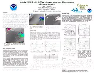
Fig. 7. (a) Vertical cross-section (at Y=500km) through region of maximum brightness temperature difference from Fig. 6. Thick lines are total condensate mixing ratio (g/kg); thin lines are temperature (K). (b) Same as (a), but thin lines are water vapor mixing ratio (g/kg). Fig. 6. (a) Horizontal cross-section of model-generated 6.185 – 10.35 µm difference. Shaded regions represent positive values. (b) Same as (a), but zoomed in and without shading. Modeling GOES-R 6.185-10.35 µm brightness temperature differences above cold thunderstorm tops Daniel T. Lindsey* NOAA/NESDIS/STAR/RAMMB Louie Grasso and Jack Dostalek Cooperative Institute for Research in the Atmosphere Introduction As the time for the launch of GOES-R approaches, it is very important that product development be well underway years before the operational data begins to arrive. To achieve this, the RAMM Branch has begun to use a cloud model with grid spacing equivalent to the GOES-R footprint to simulate actual mesoscale weather events. Output from the cloud model is then used as input to an observational operator, which generates synthetic satellite brightness temperatures at wavelengths corresponding to the Advanced Baseline Imager’s (ABI) channels. This simulated imagery can then be used to generate GOES-R products with various applications. One such case study is from 8 May 2003 in the central plains. The cloud model was initialized with ETA model initial conditions, and it subsequently produced intense thunderstorms very near where storms were observed. Fig. 1 shows the simulated 10.35 µm channel at 2100 UTC. More Model Results To have a closer look at cloud model results from the 8 May 2003 case, Fig. 6 shows the 6.185 – 10.35 µm difference over the thunderstorms in eastern Kansas. The largest value was 1.2 K. Fig. 7 shows a vertical cross-section through this maximum. Black lines denote total condensate mixing ratio, and can be interpreted as the cloud boundary. The region near x=900km is above a strong updraft and is associated with an overshooting top. Note that the largest vertical temperature gradient occurs near x=910km, and this is coincident with the maximum in brightness temperature difference in Fig. 6b. Fig. 3. Simulated 6.185 µm – 10.35 µm difference from 8 May 2003. Red pixels indicate regions of positive difference. Fig. 2. Simulated 6.185 µm channel from 8 May 2003 over the central plains. Sensitivity Tests To determine what conditions are necessary for positive 6.185 – 10.35 µm differences, a series of idealized runs were performed with the observational operator. An optically thick cloud composed of pristine ice crystals was placed so that its top was at the tropopause, or near 11,500 m AGL, at a temperature of 200 K. Three temperature profiles were formed above the tropopause, each having different temperature inversion magnitudes (Fig. 4, profiles A, B, and C). Two water vapor profiles were prescribed above the tropopause, one relatively dry and the other moist (Fig. 5, profiles “dry” and “moist”). Table 1 shows the results. Fig. 1. Simulated 10.35 µm channel from 8 May 2003 over the central plains. Intense thunderstorms can be seen over eastern Kansas. Water Vapor Difference Product Previous research by Ackerman (1996) (and others) have suggested that a positive difference between the water vapor and infrared bands is occasionally observed over thunderstorm tops. The leading hypothesis to explain these positive differences is water vapor above the very cold cloud top absorbing outgoing radiation in the 6-7 µm range, then re-radiating at a warmer temperature, since this occurs within the lower stratospheric temperature inversion. In order to investigate this idea, the observational operator discussed above was used to simulate brightness temperatures at 6.185 µm for the 8 May 2003 severe weather case. Next, a series of sensitivity tests were performed to isolate the mechanism responsible for positive brightness temperature differences. Fig. 2 shows the 6.185 µm channel, and Fig. 3 shows the difference between the 6.185 and 10.35 µm channels, where the pixels having positive differences have been colored red. These positive regions are generally co-located with thunderstorm overshooting tops. Fig. 4. Temperature profiles used for the sensitivity tests described above. Fig. 5. Water vapor profiles for the sensitivity tests Conclusions The primary purpose of this study was to demonstrate that synthetic imagery from GOES-R’s ABI can be created and analyzed, and products can be created. This particular application was chosen to explain positive differences between the 6.185 – 10.35 µm bands. To get a positive difference, it was shown that a strong vertical temperature gradient is necessary above a cold thunderstorm top. Overshooting tops tend to generate the strongest vertical temperature gradient, so positive differences are often co-located with these tops. Additionally, it is possible that either water vapor or a thin cloud layer above the thunderstorm anvil is responsible for absorbing and re-radiating the 6-7 µm radiation. Table 1. Simulated brightness temperature differences between the 6.185 and 10.35 µm channels, for temperature profiles A, B, and C, and water vapor profiles Dry and Moist. It can be seen from Table 1 that slight positive differences occur in all cases, but the magnitudes of the differences for temperature profile A (isothermal) are negligible. As the strength of the temperature inversion increases, the brightness temperature differences increase. For profile C, having a particularly moist layer above the cloud increases the brightness temperature difference by more than 2 K, but without the strong inversion, the moist layer has little effect. ------------------------------------------------------------------------------------ *Corresponding author address: 1375 Campus Delivery, CIRA/CSU, Fort Collins, CO, 80523. Lindsey@cira.colostate.edu References Ackerman, S. A., 1996: Global satellite observations of negative brightness temperature differences between 11 and 6.7 µm. J. Atmos. Sci., 53, 2803-2812.