Download
1 / 34
340 likes | 488 Views
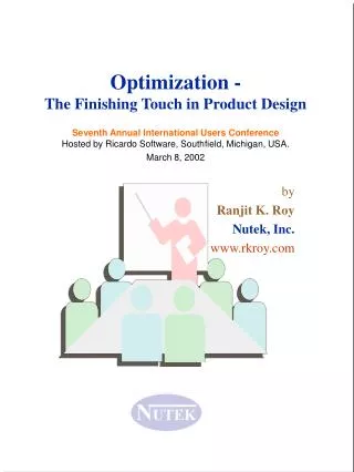
Optimization - The Finishing Touch in Product Design Seventh Annual International Users Conference Hosted by Ricardo Software, Southfield, Michigan, USA. March 8, 2002. by Ranjit K. Roy Nutek, Inc. www.rkroy.com. Introduction.

E N D
Optimization - The Finishing Touch in Product DesignSeventh Annual International Users ConferenceHosted by Ricardo Software, Southfield, Michigan, USA.March 8, 2002 by Ranjit K. Roy Nutek, Inc. www.rkroy.com
Introduction All engineering activities have roles to play in improving the product quality. Toward this goal, optimization of designs in the analytical stage presents an attractive opportunity. The statistical technique known as design of experiments (DOE), which is commonly used to experiment with prototype parts, can often be effectively utilized to optimize product designs using analytical simulations. This brief presentation offers an overview of how the Taguchi standardized form of DOE ca be applied to analytical performance models for identifying the best among the available design options. - RKR 3/8/02 Taguchi Approach - Overview
Presentation Contents • Drive & Rational for Optimization • Ultimate Goal - Robust Design • Tool for Optimization • Understanding DOE/Taguchi Approach • Industrial Applications • DOE Example - Popcorn machine optimization • Efficiencies in analytical applications • Linear model • Nonlinear model • Conclusions, Comments, and Q&A Taguchi Approach - Overview
Our Values & Rationale for Optimization • We wish to improve our products and do that we shall • ‘Leave no stone unturned’ • Seek out and settle with the best among all possible alternative design possibilities • Look for ways to optimize designs quickly and economically (Go after most benefits with least cost) Why optimize product and process designs? Reduce rework, rejects, and warranty costs. Taguchi Approach - Overview
Where do we do quality improvement? * Production * Test & Validation * Design & Development * Design & Analysis Product Engineering Roadmap (Opportunities for Building Quality) There are opportunities for improvement in all phases of product development. Taguchi Approach - Overview
Maximizing Return on Investments Where should we put our effort to optimize designs? Return on investment (ROI) is greater when efforts are made to optimize in design and analysis stages. ROI: 1 : 1 in production ROI: 1 : 10 in process design ROI: 1 : 100 in development ROI: 1 : 1000 in analyses Taguchi Approach - Overview
Do It Right The First Time! Do It Up-front In Design! Build Quality In Design! Who is Taguchi? • Genechi Taguchi was born in Japan in 1924. • Worked with Electronic Communication Laboratory (ECL) of Nippon Telephone and Telegraph Co.(1949 - 61). • Major contribution has been to standardize and simplify the use of the DESIGN OF EXPERIMENTS techniques. Taguchi Approach - Overview
What is the Design of Experiment (DOE) Technique? • It all began with R. A. Fisher in England back in 1920’s. • Fisher wanted to find out how much rain, sunshine, fertilizer, and water produce the best crop. • Design Of Experiments (DOE): • Is a statistical technique used to study effects of multiple variables simultaneously. • It helps you determines the factor combination for optimum result. Taguchi Approach - Overview
Figure 1: Performance Before Experimental Study Figure 2: Performance After Study Improve Performance = Reduce and / or Reduce m m = (Yavg - Yo ) Yavg. Yo new Looks & Measure of Improvement Taguchi Approach - Overview
Poor Quality Not so Bad Most Desirable Better Being on Target Most of the Time Taguchi Approach - Overview
How Does DOE/Taguchi Work? • Follows an experimental strategy that derives most information with minimum effort. • The technique can be applied to formulate the most desirable recipe for baking a POUND CAKE with FIVE ingredients, and with the option to take HIGH and LOW values of each. • Full factorial calls for 32 experiments. Taguchi approach requires only 8. Taguchi Approach - Overview
Factors Level-I Level-II A: Egg B: Butter C: Milk D: Flour E: Sugar Experiment Factors and their Levels FIVE factors at TWO levels each make 25 = 32 separate recipes (experimental condition) of the cake. Taguchi Approach - Overview
Orthogonal Array Experiments Work Like a Fish Finder 3 2-L factors = 8 Vs. 4 Taguchi expts. 7 ‘‘ ‘‘ = 128 8 Expts. 15 ‘‘ over 32,000 16 ‘‘ Fishing Net Taguchi Approach - Overview
Example Case Study (Production Problem Solving) I. Experiment Planning Project Title - Adhesive Bonding of Car Window Bracket An assembly plant of certain luxury car vehicle experienced frequent failure of one of the bonded plastic bracket for power window mechanism.The cause of the failure was identified to be inadequate strength of the adhesive used for the bonding. Objective & Result - Increase Bonding Strength Bonding tensile (pull) strength were going to be measured in three axial directions. Minimum force requirements were available from standards set earlier. Quality Characteristics - Bigger is better (B) Factors and Level Descriptions Bracket design, Type of adhesive, Cleaning method, Priming time, Curing temperature, etc. II. Experiment Design & Results Six different process parameters were quickly studied by experiments designed using an L-8 array. Taguchi Approach - Overview
Example Case Study# S2: (Casting Process Optimization) I. Experiment Planning Project Title - Die-Casting Process Parameter Study (CsEx-01) In a die casting process, metal (generally alloys of Aluminum, Zinc & Magnesium) parts are formed by flowing molten metals (at 1200 – 1300 deg F) in the cavities of the dies made of steel. Objective & ResultReduce Scraps Quality Characteristics - Smaller is better (S) # Criteria Descriptions Worst - Best Reading QC Rel. Wt. 1 Crack and Tear (length) 10 mm 20 mm S 20 2 Heat Sinks (diameter) 15 mm 0 mm S 30 3 Lamination (area) 5 sq.cm 0 sq.cm S 25 4 Non-Fill (area of void) 2 sq.cm 0 sq.cm S 25 Commonly Observed Characteristics There are many types of observed defects that result in scrapped parts. The common defects observed are, Surface abnormalities (Cold flaw, Cold lap, Chill swirls, Non-fill, etc.), Lamination (layers of metal on inside or outside surface), Gas Porosity, Blister, Shrinkage Porosity, Heat sinks, Crack & tears, Drags, Gate porosity, Driving ejector pins, etc. II. Experiment Design & Results An L-12 array was used to design the experiment to study 10 2-level factors. Factors are assigned to the column in random order. The results of each criteria of evaluations were analyzed separately. Taguchi Approach - Overview
Figure 1. Clutch Plate Fabrication Process Rust Inhibitor Parts are submerged in a chemical bath Stamping / Hobbing Clutch plate made from 1/16 inch thick rolled steel Deburring Clutch plates are tumbled in a large container to remove sharp edges Cleaned and dried parts are boxed for shipping. Example Case Study (Production Problem Solving) I. Experiment Planning Project Title - Clutch Plate Rust Inhibition Process Optimization Study (CsEx-05) The Clutch plate is one of the many precision components used in the automotive transmission assembly. The part is about 12 inches in diameter and is made from 1/8-inch thick mild steel. Objective & Result - Reduce Rusts and Sticky (a) Sticky Parts – During the assembly process, parts were found to be stuck together with one or more parts. (b) Rust Spots – Operators involved in the assembly reported unusually higher rust spots on the clutch during certain period in the year. Factors and Level Descriptions Rust inhibitor process parameters was the area of study. II. Experiment Design & Results One 4-level factor and four 2-level factors in this experiment were studied using a modified L-8 array. The 4-level factor was assigned to column 1 modified using original columns 1, 2, and 3. Taguchi Approach - Overview
Example Case Study # S9:( Sporting Event Optimization) I. Experiment Planning Project Title - Bow & Arrow Tuning Study There are a number of structural and geometrical factors in bow and arrow that determines how well the arrow fly. A contestant for Olympic archery competition planned to use DOE to lay out a set of experiments to determine the best bow and arrow setting for best performance. Objective & Result:Improve accuracy of hitting the bullseye. The accuracy can be measured in terms of radial distance of the hit from the center of the bullseye. Quality Characteristics: Radial distance measured in inches.Smaller is better Factors and Level Descriptions: A:Arrow Stiffness (Force required to pull the string) B:Draw Length C:Draw Weight (Force when not linearly proportional with draw length) D:Point Weight (Weight of point of arrow, steel, 90 - 110 grams) E:Plunger Button Tension (Compression force at guide - arrow rest) F:Center shot (Horizontal location of the guide) G:String Type (Plastic, Kevlar, etc.) H:Knocking Location (Location of the arrow nock on string) Interactions: AxE, ExF, AxB, & AxC II. Experiment Design & Results This experiment is designed using an L-16 array to study 8 factors and 4 interactions. Taguchi Approach - Overview
Example Case Study # S10:( Race Car Optimization) I. Experiment Planning Project Title - Race Car Suspension Parameter Optimization To achieve highest performance, major suspension parameters of race cars like those for Daytona Superspeedway (2.5 mile oval; 31 degrees banking in 1-4 turns) are fine tuned for the track. Test vehicle components can be evaluated by laying out simple experiments to determine the most desirable combination. Objective & Result: Determine the best combination of suspension parameters for the race car. Quality Characteristics: Time to complete the track. Smaller is better. Factors and Level Descriptions: (Source: USA Today, February 15, 2002) A:Right Front Tire Pressure (23 - 55 psi) Green = Superspeedway B:Left Front Tire Pressure (15 - 30 psi) C:Right Rear Tire Pressure (20 - 50 psi) D:Left Rear Tire Pressure (15 - 30 psi) E:Right Front Spring Rate (1,900 - 800 lbs/in) F:Left Front Spring Rate (700 - 800 lbs/in) G:Right Rear Spring Rate (225 - 350 lbs/in) H:Left Rear Spring Rate (15 - 30 lbs/in) I:Rear Spoiler Angle (0 - 55 degrees) II. Experiment Design & Results Up to 11 factors as shown above can be studied by designing an experiment using an L-12 array. Taguchi Approach - Overview
[Example DOE]Popcorn Machine(Example application. Not included in seminar handout.) • An ordinary kernel of corn, a little yellow seed, it just sits there. But add some oil, turn up the heat, and, pow. Within a second, an aromatic snack sensation has come into being: a fat, fluffy popcorn. Note: C. Cretors & Company in the U.S. was the first company to develop popcorn machines, about 100 years ago. Taguchi Approach - Overview
I. Experiment Planning • Title of Project - Pop Corn Machine performance Study • Objective & Result - Determine best machine settings • Quality Characteristics - Measure unpopped kernels (Smaller is better) Factors and Level Descriptions Notation Factor Description Level I Level II A: Hot Plate Stainless Steel Copper Alloy B: Type of Oil Coconut Peanut C: Heat Setting Setting 1 Setting 2 Taguchi Approach - Overview
Orthogonal Arrays for Common Experiment Designs Use this array (L-4) to design experiments with three 2-level factors Use this array (L-8) to design experiments with seven 2-level factors L4 (23) Array Cols>> Trial# 1 2 3 1 1 1 1 2 1 2 2 3 2 1 2 4 2 2 1 L8(27 ) Array Cols.>> TRIAL# 1 2 3 4 5 6 7 1 1 1 1 1 1 1 1 2 1 1 1 2 2 2 2 3 1 2 2 1 1 2 2 4 1 2 2 2 2 1 1 5 2 1 2 1 2 1 2 6 2 1 2 2 1 2 1 7 2 2 1 1 2 2 1 8 2 2 1 2 1 1 2 L9(34) Trial/Col# 1 2 3 4 1 1 1 1 1 2 1 2 2 2 3 1 3 3 3 4 2 1 2 3 5 2 2 3 1 6 2 3 1 2 7 3 1 3 2 8 3 2 1 3 9 3 3 2 1 Use this array (L-9) to design experiments with four 3-level factors Taguchi Approach - Overview
II. Experiment Design & Results # C A B Results (oz)* 1 1 1 1 5 2 1 2 2 8 3 2 1 2 7 4 2 2 1 4 Design Layout (Recipes) Expt.1: C1 A1 B1 or [Heat Setting 1, Stainless Steel Plate, & Coconut Oil ] Expt.2: C1 A2 B2 or [Heat Setting 1, Copper Plate, & Peanut Oil ] Expt.3: C2 A1 B2 or [Heat Setting 2, Stainless Steel Plate, & Peanut Oil ] Expt.4: C2 A2 B1 or [Heat Setting 2, Copper Plate, & Coconut Oil ] How to run experiments: Run experiments in random order when possible Taguchi Approach - Overview
Calculations: ( Min. seven, 3 x 2 + 1) (5 + 8 + 7 + 4 ) / 4 = 6 (5 + 8) / 2 = 6.5 (7 + 4) / 2 = 5.5 (5 + 7) / 2 = 6.0 (8 + 4) / 2 = 6.0 (5 + 4) / 2 = 4.5 (8 + 7) / 2 = 7.5 _ T = _ C1 = _ C2 = _ A1 = _ A2 = _ B1 = _ B1 = 9 Main Effects (Average effects of factor influence) 8 7 6 UNPOPPED KERNELS 5 4 3 A1 Hot plate A2 B1 OilB2 C1 Heat SettingC2 III. Analysis of Results • Trend of Influence: • How do the factor behave? • What influence do they have to • the variability of results? • How can we save cost? • Optimum Condition: • What condition is most desirable? Taguchi Approach - Overview
Yopt= + + + = 6.0 + ( 6 – 6 ) + (4.5 – 6.0 ) + ( 5.5 – 6.0 ) = 4.0 _ T __ A1 + _ ( A1 + _ ( C2 + _ ( B1 + _ T ) _ T ) _ T ) III. Analysis of Results (contd.) • Expected Performance: • What is the improved performance? • How can we verify it? • What are the boundaries of expected performance? (Confidence Interval, C.I.) • Notes: • Generally, the optimum condition will not be one that has already been tested. Thus you will need to run additional experiments to confirm the predicted performance. • Confidence Interval (C.I.) on the expected performance can be calculated from ANOVA calculation. These boundary values are used to confirm the performance. Taguchi Approach - Overview
Analytical Simulations With Seven FactorsA process performance (Y) which is dependent on seven factors (A, B, C, ...) can be represented by many types of mathematical functions as shown here. Linear: Y = C1*A + C2*B + C3*C + C4*D + C5*E + C6*F + C7*GHyperbolic: Y = 100*(C1+C2+C3+C4+C5+C6+C7)/(A+B+C) + (D+E)/(F+G) Polynomial: Y = C1*A + C2*B^2 + C3*C^2 + C4/D^3 + C5*E/(F + G)^2 Complex: Y = 0.50 - ((A + B + C) * D^3) / (4000 * E * F * G^3) Logarithmic:Y = 10 * LOG((C1/A^5 + C2/B^4 + C3*C^3 + C4*D^2 + C5*E^3 + C6*F*C7*G) / 1000) Linear Equation:(constants assumed) Y = 0.02*A + 0.001*B + 0.0001*C + 0.04*D + 1.5*E + 21.6*F + 12.7*G Factors A B C D E F G Level 1 2500 1900 4000 32.0 29.5 6.90 10.5 Level 2 2650 1520 4800 30.0 30.7 7.80 11.4 Full Factorial Experiments (All possible combinations (* Taguchi L-8 conditions) ) # Description Results # Description Results 1 1 1 1 1 1 1 1 380.220* 2 1 1 1 1 1 1 2 391.650 3 1 1 1 1 1 2 1 399.660 4 1 1 1 1 1 2 2 411.090 5 1 1 1 1 2 1 1 382.020 6 1 1 1 1 2 1 2 393.450 7 1 1 1 1 2 2 1 401.460 8 1 1 1 1 2 2 2 412.890 9 1 1 1 2 1 1 1 380.140 10 1 1 1 2 1 1 2 391.570 11 1 1 1 2 1 2 1 399.580 12 1 1 1 2 1 2 2 411.010 13 1 1 1 2 2 1 1 381.940 14 1 1 1 2 2 1 2 393.370 15 1 1 1 2 2 2 1 401.380 16 1 1 1 2 2 2 2 412.810* 17 1 1 2 1 1 1 1 380.300 18 1 1 2 1 1 1 2 391.730 19 1 1 2 1 1 2 1 399.740 20 1 1 2 1 1 2 2 411.170 Taguchi Approach - Overview
21 1 1 2 1 2 1 1 382.100 22 1 1 2 1 2 1 2 393.530 23 1 1 2 1 2 2 1 401.540 24 1 1 2 1 2 2 2 412.970 25 1 1 2 2 1 1 1 380.220 26 1 1 2 2 1 1 2 391.650 27 1 1 2 2 1 2 1 399.660 28 1 1 2 2 1 2 2 411.090 29 1 1 2 2 2 1 1 382.020 30 1 1 2 2 2 1 2 393.450 31 1 1 2 2 2 2 1 401.460 32 1 1 2 2 2 2 2 412.890 33 1 2 1 1 1 1 1 379.840 34 1 2 1 1 1 1 2 391.270 35 1 2 1 1 1 2 1 399.280 36 1 2 1 1 1 2 2 410.710 37 1 2 1 1 2 1 1 381.640 38 1 2 1 1 2 1 2 393.070 39 1 2 1 1 2 2 1 401.080 40 1 2 1 1 2 2 2 412.510 41 1 2 1 2 1 1 1 379.760 42 1 2 1 2 1 1 2 391.190 43 1 2 1 2 1 2 1 399.200 44 1 2 1 2 1 2 2 410.630 45 1 2 1 2 2 1 1 381.560 46 1 2 1 2 2 1 2 392.990 47 1 2 1 2 2 2 1 401.000 48 1 2 1 2 2 2 2 412.430 49 1 2 2 1 1 1 1 379.920 50 1 2 2 1 1 1 2 391.350 51 1 2 2 1 1 2 1 399.360 52 1 2 2 1 1 2 2 410.790* 53 1 2 2 1 2 1 1 381.720 54 1 2 2 1 2 1 2 393.150 55 1 2 2 1 2 2 1 401.160 56 1 2 2 1 2 2 2 412.590 57 1 2 2 2 1 1 1 379.840 58 1 2 2 2 1 1 2 391.270 59 1 2 2 2 1 2 1 399.280 60 1 2 2 2 1 2 2 410.710 61 1 2 2 2 2 1 1 381.640* 62 1 2 2 2 2 1 2 393.070 63 1 2 2 2 2 2 1 401.080 64 1 2 2 2 2 2 2 412.510 65 2 1 1 1 1 1 1 383.220 66 2 1 1 1 1 1 2 394.650 67 2 1 1 1 1 2 1 402.660 68 2 1 1 1 1 2 2 414.090 69 2 1 1 1 2 1 1 385.020 70 2 1 1 1 2 1 2 396.450 71 2 1 1 1 2 2 1 404.460 72 2 1 1 1 2 2 2 415.890 73 2 1 1 2 1 1 1 383.140 74 2 1 1 2 1 1 2 394.570 75 2 1 1 2 1 2 1 402.580 76 2 1 1 2 1 2 2 414.010 77 2 1 1 2 2 1 1 384.940 78 2 1 1 2 2 1 2 396.370 Taguchi Approach - Overview
79 2 1 1 2 2 2 1 404.380 80 2 1 1 2 2 2 2 415.810 81 2 1 2 1 1 1 1 383.300 82 2 1 2 1 1 1 2 394.730 83 2 1 2 1 1 2 1 402.740 84 2 1 2 1 1 2 2 414.170 85 2 1 2 1 2 1 1 385.100 86 2 1 2 1 2 1 2 396.530* 87 2 1 2 1 2 2 1 404.540 88 2 1 2 1 2 2 2 415.970 <= Highest value 89 2 1 2 2 1 1 1 383.220 90 2 1 2 2 1 1 2 394.650 91 2 1 2 2 1 2 1 402.660* 92 2 1 2 2 1 2 2 414.090 93 2 1 2 2 2 1 1 385.020 94 2 1 2 2 2 1 2 396.450 95 2 1 2 2 2 2 1 404.460 96 2 1 2 2 2 2 2 415.890 97 2 2 1 1 1 1 1 382.840 98 2 2 1 1 1 1 2 394.270 99 2 2 1 1 1 2 1 402.280 100 2 2 1 1 1 2 2 413.710 101 2 2 1 1 2 1 1 384.640 102 2 2 1 1 2 1 2 396.070 103 2 2 1 1 2 2 1 404.080* 104 2 2 1 1 2 2 2 415.510 105 2 2 1 2 1 1 1 382.760 106 2 2 1 2 1 1 2 394.190* 107 2 2 1 2 1 2 1 402.200 108 2 2 1 2 1 2 2 413.630 109 2 2 1 2 2 1 1 384.560 110 2 2 1 2 2 1 2 395.990 111 2 2 1 2 2 2 1 404.000 112 2 2 1 2 2 2 2 415.430 113 2 2 2 1 1 1 1 382.920 114 2 2 2 1 1 1 2 394.350 115 2 2 2 1 1 2 1 402.360 116 2 2 2 1 1 2 2 413.790 117 2 2 2 1 2 1 1 384.720 118 2 2 2 1 2 1 2 396.150 119 2 2 2 1 2 2 1 404.160 120 2 2 2 1 2 2 2 415.590 121 2 2 2 2 1 1 1 382.840 122 2 2 2 2 1 1 2 394.270 123 2 2 2 2 1 2 1 402.280 124 2 2 2 2 1 2 2 413.710 125 2 2 2 2 2 1 1 384.640 126 2 2 2 2 2 1 2 396.070 127 2 2 2 2 2 2 1 404.080 128 2 2 2 2 2 2 2 415.510 The Maximum Y is 415.97 at condition # 88 (88 2 1 2 1 2 2 2 415.970 ). Taguchi Approach - Overview
Calculated Results Based on Conditions Defined by an L-8 Array Design TRIAL# A B C D E F G Results Comb.# 1 1 1 1 1 1 1 1 380.220 # 1 2 1 1 1 2 2 2 2 412.810 # 16 3 1 2 2 1 1 2 2 410.790 # 52 4 1 2 2 2 2 1 1 381.640 # 61 5 2 1 2 1 2 1 2 396.530 # 86 6 2 1 2 2 1 2 1 402.660 # 91 7 2 2 1 1 2 2 1 404.080 # 103 8 2 2 1 2 1 1 2 394.190 # 106 From full factorial (analytical simulation): Highest value from L-8 design: 415.966, which compares with # 88 2 1 2 1 2 2 2 415.970 <= 100% accurate Taguchi Approach - Overview
Analytical Simulation with Nonlinear (Complex) Equation Complex Equation: Y = 0.50 - ((A + B + C) * D^3) / (4000 * E * F * G^3) Factors A B C D E F G Level 1 2500 1900 4000 32.0 29.5 6.90 10.5 Level 2 2650 1520 4800 30.0 30.7 7.80 11.4 Calculations of Y for all possible conditions (128) produce... …... 46 1 2 1 2 2 1 2 0.328 47 1 2 1 2 2 2 1 0.305 48 1 2 1 2 2 2 2 0.347 Highest value Taguchi Approach - Overview
Calculated Results Based on Conditions Defined by an L-8 Array Design TRIAL# A B C D E F G Results Comb. # 1 1 1 1 1 1 1 1 0.208 # 1 2 1 1 1 2 2 2 2 0.340 # 16 3 1 2 2 1 1 2 2 0.288 # 52 4 1 2 2 2 2 1 1 0.257 # 61 5 2 1 2 1 2 1 2 0.256 # 86 6 2 1 2 2 1 2 1 0.263 # 91 7 2 2 1 1 2 2 1 0.259 # 103 8 2 2 1 2 1 1 2 0.317 # 106 From full factorial (analytical simulation): #48 1 2 1 2 2 2 2 0.347 , which compares with O.35. <= Highly accurate. Taguchi Approach - Overview
Conclusions and Comments • Most optimization studies tend to involves unnecessary complications that is not cost effective. • Simpler DOE/Taguchi with focus on robustness produce the most benefit. • Most optimization technique would work well for most jobs when applied with proper understanding of the application principles. • Automation in analysis is not a substitute for knowledge of science and physics. Thank you for attending- Ranjit K. Roy Taguchi Approach - Overview
Thoughts for the day . . One morning, having moved into a new neighborhood, the family noticed that the school bus didn't show up for their little boy. The dad volunteered saying, “I will drive you, if you show me the way”. On their way the young student directed dad to turn right, then a left, and a few more lefts and rights. Seeing that the school was within a few blocks from home, dad asked, “Why did you make me drive so long to get to the school this close to home”. The boy replied, “But dad, that’s how the school bus goes everyday”. - Mort Crim, WWJ 950 Radio, Detroit, MI, 10/30/01 “When you always do what you always did, you will always get what you always got” Taguchi Approach - Overview
QT4 Nutek, Inc.3829 Quarton RoadBloomfield Hills, MI 48302, USA.Tel: 1-248-5404827, E-mail: rkroy@rkroy.comhttp://www.rkroy.com Training & Workshop, Assistance with application, Books and Software for Design of Experiments Using The Taguchi Approach
Nature of Nutek Training Services • Seminar with hands-on application workshop (Taguchi Approach) [Our seminar, books, & software use consistent notations and terminology. Class lecture focuses on application, with most discussions on method rather than the math.] • Length of training - This 4-day training consists of two days of class room seminar and two days of hands-on computer workshop, during which the attendees learn how to apply the technique in their own projects. • Training objectives - Teach attendees the application methodologies & prepare them for immediate applications.