Multisource Full Waveform Inversion of Marine Streamer Data with Frequency Selection
250 likes | 388 Views
Multisource Full Waveform Inversion of Marine Streamer Data with Frequency Selection. Yunsong Huang and Gerard Schuster KAUST. Goal of the study Multisource Mismatch solution with marine data Low-discrepancy frequency coding Numerical results Conclusions. Outline.

Multisource Full Waveform Inversion of Marine Streamer Data with Frequency Selection
E N D
Presentation Transcript
Multisource Full Waveform Inversion of Marine Streamer Data with Frequency Selection YunsongHuang and Gerard Schuster KAUST
Goal of the study Multisource Mismatch solution with marine data Low-discrepancy frequency coding Numerical results Conclusions Outline
Goal of the Study Multisource optimization for marine FWI Standard optimization for FWI Speed and quality comparison
Aim of the study Multisource Migration Least Squares Multisource Migration Low-discrepancy frequency coding Numerical results Conclusions Outline
Standard Migration vs Multisource Migration Romero, Ghiglia, Ober, & Morton, Geophysics, (2000) Given: d1 and d2 Given: d1+ d2 Find: m Find: m Soln: m = (L1 + L2)(d1+d2) T T T Soln: m=L1 d1 + L2 d2 T T = L1 d1 + L2 d2 Benefit: Reduced computation and memory Liability: Crosstalk noise … T T + L1 d2 + L2 d1 Src. imaging cond. xtalk
Multisource LSM & FWI Inverse problem: 1 ~ ~ m || d – L m ||2 arg min J = 2 Dd misfit Iterative update: ~T m(k+1) = m(k) + aLDd K=1 T T L1Dd1+ L2Dd2 K=10 T T + L1 Dd2+ L2 Dd1
Brief Early History Multisource Phase Encoded Imaging Migration Romero, Ghiglia, Ober, & Morton, Geophysics, (2000) Waveform Inversion and Least Squares Migration Krebs, Anderson, Hinkley, Neelamani, Lee, Baumstein, Lacasse, SEG Zhan+GTS, (2009) Virieux and Operto, EAGE, (2009) Dai, and GTS, SEG, (2009) Biondi, SEG, (2009)
Aim of the study Multisource Migration Mismatch solution with marine data Low-discrepancy frequency coding Numerical results Conclusions Outline
Land Multisource FWI Fixed spread Simulation geometry must be consistent with the acquisition geometry
Marine Multisource FWI Mismatch solution with marine data Observed marine data purify Freq. encoding Decode & mute Simulated land data 4 Hz 4 Hz 4 Hz 8 Hz 8 Hz 8 Hz F.T., freq. selec. wrong misfit Blend 4 Hz 8 Hz
Multisource FWI Freq. Sel. Workflow Select unique frequency for each src dd For k=1:K Filter and blend observed data: dd dpreddpred Purify predicted data: dpreddpred Data residual: Dd=dpred-d ~T m(k+1) = m(k) + aLDd end
Aim of the study Multisource Mismatch solution with marine data Low-discrepancy frequency coding Numerical results Conclusions Outline
Low-discrepancy Frequency Encoding Standard Low-discrepancy 60 encoding encoding 60 60 Frequency index Frequency index Frequency index 1 Source index Source index 60 60 1 1 1 1
Aim of the study Multisource Mismatch solution with marine data Low-discrepancy frequency coding Numerical results Conclusions Outline
Frequency-selection FWI of 2D Marine Data 0 • Shots: 60 • Source freq: 8 Hz • Receivers/shot: 84 Z (km) • Cable length: 2.3 km 4.5 (km/s) 1.5 1.5 6.8 X (km) 0
FWI images 0 0 • Actual model • Starting model Z (km) Z (km) 1.5 1.5 • Standard FWI • (69 iterations) • Multisource FWI • (262 iterations) 6.8 6.8 X (km) X (km) 0 0
Convergence Rates Waveform error Faster initial convergence rate of the white curve 1 1 supergather, standard encoding Same asymptotic convergence rate of the red and white curves Log normalized by individual sources 3.8x 1 supergather, low-discrepancy encoding 0.025 69 1 262 Log iterationnumber
Convergence Rates Speedup 60 / 2 / 2 / 3.8 = 4 Velocity error 1 • Gain • 60: sources • Overhead factors: • 2 x FDTD steps • 2 x domain size • 3.8 x iteration number 1 supergather, standard encoding Log normalized by individual sources 3.8x 1 supergather, low-discrepancy encoding 0.35 69 1 262 Log iterationnumber
Convergence Rates Velocity error (normalized) Low-discrepancy encoding is 12% to 3x faster initially than Standard encoding 1 standard encoding 10 0.75 1 iterationnumber
Frequency selection is implemented in FDTD 2 x time steps per forward or backward modeling Low-discrepancy frequency encoding affects no asymptotic rate of convergence helps to reduce model error in the beginning of simulation 4x speedup for the multisource FWI on the synthetic marine model Conclusions
Thanks Sponsors of the CSIM (csim.kaust.edu.sa) consortium at KAUST & KAUST HPC
At lower (say 1/2) frequencies, the frequency selection strategy sees fewer frequency resources, but Computation cost: (Nx x Nz) x Ns x Nt is reduced by 1/16, since each factor is halved. This part does not degrade the overall speedup much. In the case of multiscale
Convergence Rates Slew rate = H/L Velocity error (normalized) L 1 1 supergather, standard encoding H by individual sources 1 supergather, low-discrepancy encoding 0.75 1 10 iterationnumber