Download
1 / 50
550 likes | 826 Views
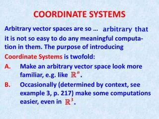
cts. cts. Motor#1 (10,000 ). Motor#2 (10,000 ). in. in. Power PMAC Coordinate Systems December 2013. Y(in). #1->10000.00X-2.91Y #2->10000.00Y. X(in). 1 arc min (exaggerated). Power PMAC Coordinate Systems. Main structure for providing multi-axis coordination

E N D
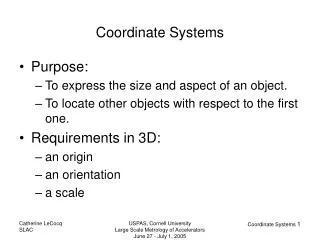
cts cts Motor#1 (10,000 ) Motor#2 (10,000 ) in in Power PMAC Coordinate SystemsDecember 2013 Y(in) #1->10000.00X-2.91Y #2->10000.00Y X(in) 1 arc min (exaggerated)
Power PMAC Coordinate Systems • Main structure for providing multi-axis coordination • Same scheme as Turbo PMAC, but enhanced capabilities • Axes to start, stop, and change speed at same time should be in the same coordinate system • Axes to act independently should be in separate coordinate systems • Axes to share faults should be in the same coordinate system • Key concept: mapping of motors (actuators) to axes (programming coordinates) • Two methods of defining coordinate systems: • Axis definition statements • For mathematically linear mappings of motors to axes • Forward and inverse kinematic subroutines • Typically for mathematically non-linear mappings of motors to axes • Useful for non-Cartesian machine geometries
Coordinate System Numbering • Coordinate system numbers start at zero (&0) • User sets maximum number of coordinate systems supported with Sys.MaxCoords • Default value is 16, maximum value is 128 • Highest usable C.S. number is (Sys.MaxCoords – 1) • Setting larger than necessary adds to backup file size, some to CPU load • It is expected that most users will not employ CS 0 (&0) as a “real” CS • On re-initialization, all motors have “null” definition in CS 0 • &0 addressed by default at power-on/reset • &x data structure elements use Coord[x].{element name} • “Legacy” I-variable support for existing functions in CS 0 – 15 • I5000 – 5099 for CS 0 (not for data gathering variables) • I5100 – 5199 for CS 1 … • I6500 – 6599 for CS 15
Power PMAC Axis Attributes • Up to 32 independent axes in a single coordinate system • Existing axis names A, B, C, U, V, W, X, Y, Z • Additional axis names AA, BB, …, ZZ (excluding II, JJ, KK) • II, JJ, KK are vector names for XX/YY/ZZ 3D-space • Real-time scaling and offset for all axes • Special properties for X/Y/Z and XX/YY/ZZ spaces • Circular interpolation on any plane in the 3D space • Tool radius compensation on any plane in the X/Y/Z space • Special properties for X/Y/Z, XX/YY/ZZ, U/V/W, UU/VV/WW spaces • Real-time 3x3 matrix transformations of the space • Special properties for A, B, C, AA, BB, CC axes • Programmed rollover as rotary axes • Multiple motors can be assigned to the same axis (e.g. gantry) • Virtual axes can be used (not assigned to any motor)
Power PMAC Axis Definition Statements • Easiest way of assigning motors to axes • Suitable for most simple machine geometries • Map motor to axis (or axes) in a coordinate system with (optional) scaling and offset – scaling defines axis units • Usually one-to-one mapping of motors to axes • e.g. &1 #1->1000X, #2->1000Y • Each motor can be defined as a linear combination of up to 32 axes • e.g.: #4->1000A+250V-33.333333GG+0.00005 • Note that combinations are not just limited to XYZ and UVW “triplets”, as in PMAC and Turbo PMAC • Multiple identical definitions are permitted, as for gantries • e.g. &1 #1->X, #2->X • One motor cannot be assigned to two separate axes • e.g. &1 #1->X, #1->Y is not valid (2nd definition overwrites 1st) • e.g. &1 #1->X, &2 #1->X is not valid (2nd definition is rejected)
The “Null” Axis Definition • &m #n->0 “null” definition means that Motor n will not (directly) use any axis’ command trajectory • This motor will use C.S. m time base value • This motor will be stopped on fault of other motor in C.S. m • By default, all motors have the null definition in C.S. 0 (&0 #n->0) • Motors whose definition is never changed will use C.S. 0’s time base • The undefine all command gives all motors this null definition in C.S. 0 • A motor with a null definition in one C.S. may be redefined as an axis in another C.S. • A motor with a real axis definition in one C.S. must first get null definition in that C.S. before redefinition to another C.S. • The null definition is useful for “gantry follower” motors • This mode enabled by Motor[x].ServoCtrl = 8 (not 1 as for most motors) • Motors in this mode use trajectory from other motor as specified by Motor[x].CmdMotor – this should be number of “gantry leader” motor
The “Spindle” Axis Definition • &m #n->S[{constant}] definition assigns Motor n as a spindle axis in Coordinate System m • Does not use any axis’ command trajectory • Can be killed or aborted on fault of other motor in C.S. m • Spindle axis can be commanded separately from other axes in C.S. m • e.g. jog command for closed-loop velocity control • e.g. out command for open-loop velocity control • Intended for motor sometimes used as positioning axis • Do not need to redefine lookahead buffer when changing between positioning and spindle axis • If motor always used as spindle, do not need this definition (!) • Three ways of defining a spindle axis • &m #n->S – uses C.S. m’s % time base value • &m #n->S0 – uses C.S. 0’s % time base value • &m #n->S1 – uses fixed %100 time base value • Does not use segmentation override value in any case
Rotary Axis Position Rollover • Permits ease of programming of continuously rotatable axes • Supported for A, B, C, AA, BB, CC axes in each C.S. only • Used for abs mode moves only • Can be used with kinematic-routine axis definitions • Implemented with saved elements Coord[x].PosRollOver[i] • i= 0 .. 5 for A, B, C, AA, BB, CC axes, respectively • Note that these are axis variables (in axis user units), not motor variables as they were in PMAC/Turbo PMAC = 0.0 (default) disables rollover > 0.0, specifying cycle size (usually = 360) enables “short path” rollover • No abs move distance > ½ cycle < 0.0, specifying -cycle size (usually = -360) enables “sign-is-direction” rollover • Magnitude is destination angle, sign sets direction to this angle • No abs move distance > 1 cycle • Resulting axis (and motor) position does not roll over • Must use “modulo” (remainder) math to report position within one cycle
Axis Rollover Examples • (Starting point in program) ABS // Absolute mode A315 // Previous move • Coord[x].PosRollover[0]=0.0(rollover disabled) A45 // Takes path 1 • Coord[x].PosRollover[0]=360(short-direction rollover enabled) A45 // Takes path 2 • Coord[x].PosRollover[0]=-360(sign-is-direction rollover enabled) A45 // Takes path 2 • Coord[x].PosRollover[0]=-360(sign-is-direction rollover enabled) A-45 // Takes path 1
Power PMAC “Position Match” • Technically, the set of axis definition statements for a coordinate system constitute a matrix to convert from axis to motor coordinates • This matrix must be inverted to convert from motor to axis positions • Required to start programmed moves from arbitrary position, or when matrix is changed • Desirable for reporting of position, etc. in axis coordinates • Power PMAC automatically performs this matrix inversion for axis reporting functions and when starting motion programs • Inside motion program, starting axis positions for a move are ending axis positions of previous move • Not automatically done when commanding axis moves from PLC program, or when definitions, transformations changed within program • Changing position-following mode (Motor[x].MasterCtrl bit 1) requires position match before next move • Can be commanded explicitly with pmatch command (on-line or buffered)
Power PMAC “Position Match” Special Cases • Generally, axis-definition matrix inversion is straightforward (and invisible to user) • Some special cases must be (and are!) handled • More motors than axes (e.g. gantry) require decision • In case of identical definitions, lower-numbered motor used • In case of cross-coupling with more motors than axes, most “orthogonal” (mathematically) motors used • User can override default decision as to which motors to use (by changing Motor[x].Csolve bits); this is very rare • Non-invertible cases cause error • More axes than motors (e.g. #1->X+Y only) • Identical definitions reduce effective number of motors (e.g. #1->X+Y, #2->X+Y) • Cannot start motion program or report axis position in these cases (status bit Coord[x].Csolve = 0)
Power PMAC Kinematic Routines • Alternative, algorithmic method for mapping motors and axes in coordinate system • Permits mathematically non-linear motor/axis mappings • Commonly used for non-Cartesian mechanisms • Allows user programming of tool-tip position and path • Written in Script language (but can call C subroutine) • Forward-kinematic (FK) routine converts motor (“joint”) positions to axis (“tool-tip”) positions • Executed whenever pmatch is required (automatic or explicit) • Inverse-kinematic (IK) routine converts axis to motor positions • Executed each programmed move, or each segment for path • If forward-kinematic routine exists, it will be used, even if axis-definition statements determine inverse kinematics • If any motor in CS is defined as inverse-kinematic axis, all forward kinematics must be done in routine
Power PMAC Kinematic Routines (cont.) • Each coordinate system can have a forward-kinematic and an inverse-kinematic subroutine • FK routine must compute all axis positions in CS given motor positions • IK routine must compute motor positions for all CS motors defined as IK axes (e.g. #1->I); other motor positions can use axis-definition equations (not recommended) • User’s responsibility to ensure that FK and IK routines are proper inverses of each other over entire workspace • If they don’t agree, will get a sudden jump at the start of a program! • FK and IK subroutines written in Power PMAC script language • Subroutines use local variables, so can be reused • Same FK routine is used for starting-position calculation and axis position/velocity/following-error reporting • Iterative routines permitted – Ldata.GoBack (default = 10) limits loops before error
Forward Kinematic Routine Variable Passing • Uses CS or command-processor local (L & C) variables • Input value of Ln (n = 0 to Sys.MaxMotors-1) is position of Motor n • Input value of D0 > 0 specifies request for double calculation • Power PMAC sets these automatically on entry • Returned value of Cn (n = 0 to 31) is scaled position of axis • User must calculate and assign these values before exit • C0 to C8 for A,B,C,U,V,W,X,Y,Z respectively • C9 to C16 for AA,BB,…,HH respectively • C17 to C31 for LL, MM, …, ZZ respectively • {C0 is same as L(Sys.MaxMotors), C1 as L(Sys.MaxMotors+1)} • Returned D0 value is mask specifying which axes have been calculated • User must set each time executed (usually constant for an application) • Bit n of D0 corresponds to Cn calculated • e.g. D0=$1C0 (bits 6, 7, & 8 = 1) for X, Y, and Z calculated • Power PMAC automatically uses mask-specified Cn values as axis positions
Forward Kinematic “Double Pass” Option • Needed for axis velocity (&nv) and following error (&nf) reporting • These require transforms of two values each (new and old position for v, desired and actual position for f) • If input value of D0 (automatically set by Power PMAC) > 0, Power PMAC wants 2 passes through FK calculations • 2nd pass must “push” stack of local variables – use callsub to invoke • Best handled as follows: open forward if (D0 > 0) callsub 100; // So two passes if requested D0 = {axes-calculated mask} // Note different use of D0 for return N100: {single pass of FK calculations} return; close
Inverse Kinematic Routine Variable Passing • Uses CS local (L & C) variables • Input value of Cn (n = 0 to 31) is scaled position of axis • Power PMAC sets these automatically on entry • C0 to C8 for A,B,C,U,V,W,X,Y,Z respectively • C9 to C16 for AA,BB,…,HH respectively • C17 to C31 for LL, MM, …, ZZ respectively • {C0 is same as L(Sys.MaxMotors), C1 as L(Sys.MaxMotors+1)} • Returned value Ln (n = 0 to Sys.MaxMotors-1) is position of Motor n • User must calculate and assign these values for all #n->I motors • If input value of D0 != 0, then should process velocities also (rarely used) • Power PMAC sets D0 to 1 for PVT mode (non-segmented) • Input axis velocities in C32 – C63 (32 greater than C-var # for axis position) • Return motor velocities in “matching” Rn variables (same # as L-var) • Power PMAC automatically uses Ln values for IK motors as position (and Rn values as velocity if specified)
Example Simple Kinematic Routines(No variable substitutions) • To implement equivalent of &1 #1->1000X, #2->1000Y • Forward-kinematic routine: &1 open forward if (D0 > 0) callsub 100; // Double pass for velocity or error calcs D0=$C0; // X and Y positions set (bits 6 & 7 = 1) N100: C6=L1/1000; // Xpos=Mtr1pos/1000 C7=L2/1000; // Ypos=Mtr2pos/1000 close • Inverse-kinematic routine (used with axis definitions &1 #1->I, #2->I): &1 open inverse L1=C6*1000; // Mtr1pos=Xpos*1000 L2=C7*1000; // Mtr2pos=Ypos*1000 if (D0 > 0) { // True for unsegmented PVT only R1=C38*1000; // Mtr1vel=Xvel*1000 R2=C39*1000; // Mtr2vel=Yvel*1000 } close
Kinematic Routine IDE Variable Names • Useful for making easily understandable code • Predefined set of text substitutions • Substitutions automatically performed during download by IDE • KinPosMotorn for Ln {Motor n kinematic position} • KinVelMotorn for Rn {Motor n kinematic velocity} • KinPosAxisα for Cn {Axis α kinematic position} • n = 0 for A, 1 for B, 2 for C, 3 for U, etc. • KinVelAxisα for C(n+32) {Axis α kinematic velocity} • KinAxisUsed for D0 {Bit mask output for axes used in FK} • KinVelEna for D0 {Boolean input for IK and FK}
Two-Link Robot Arm Kinematic Equations • Forward kinematic equations • Inverse kinematic equations
Two-Link Robot Arm Kinematics Example open forward if(Coord[1].HomeComplete){ // All motors referenced? if (KinVelEna) callsub 100; // Double pass for vel calcs? KinAxisUsed=$C0; // X&Y returned N100: // Start of calculations KinPosAxisX=Len1*cosd(KinPosMotor1) +Len2*cosd(KinPosMotor1+KinPosMotor2-90); KinPosAxisY=Len1*sind(KinPosMotor1) +Len2*sind(KinPosMotor1+KinPosMotor2-90); // Pre-compute terms for inv kin SumLenSqrd=Len1*Len1+Len2*Len2; ProdofLens=2*Len1*Len2; DifLenSqrd=Len1*Len1-Len2*Len2; } else abort1; // Not referenced; stop close
Two-Link Robot Arm Kinematics Example open inverse X2Y2=pow(KinPosAxisX,2)+pow(KinPosAxisY,2); // X^2 + Y^2 Bcos=(X2Y2-SumLenSqrd)/ProdofLens; // cos(B) if (abs(Bcos)<0.9995){ // Valid solution? KinPosMotor2=acosd(Bcos)+90; // B motor angle AplusC=atan2d(KinPosAxisY,KinPosAxisX); Cangle=acosd(((X2Y2+DifLenSqrd) / (2*Len1*sqrt(SumLenSqrd)); KinPosMotor1=AplusC-Cangle; // A motor angle } else abort1; // No valid solution, stop close
Potential Issues with Inverse Kinematics • Multiple solutions possible for given tool-tip coordinates • Usually manifested as +/- sqrt, +/-acos solutions • Subroutine must explicitly select which solution is used • Transition from one solution “zone” to another • May not be possible along path of desired move • Moves may need to be restricted to one solution zone • Special operational mode may be needed to transition between zones • Singularity positions • Infinite number of solutions possible at exact singularity • Joint velocities and accelerations can be very high near singularity • No solutions possible for given tool-tip coordinates • Tool-tip coordinates not within valid workspace • Usually manifested as function domain error (e.g. sqrt(-X)) • Possible in middle of move even when end points are valid • Subroutine must explicitly handle, usually by aborting program
Axis Data Reporting • Power PMAC can report key axis data in response to host on-line query commands • &xp: Report axis actual positions for specified CS (&x) • &xd: Report axis desired positions for specified CS (&x) • &xf: Report axis following errors for specified CS (&x)* • &xv: Report axis (filtered) velocities for specified CS (&x)* • No modal CS addressing for these commands – if no &x immediately preceding command, will report for addressed motor • Data provided in axis user units with axis names • For all axes assigned to motor in this CS (e.g. X6.001 Y3.995 Z2.533) • Power PMAC performs forward kinematic calculations from present motor data, using: • Inversion of axis-definition matrix, or • User-supplied forward-kinematic subroutine (if present) • Also, inverse of axis-transformation matrix, if one is selected for C.S. • Error reported if cannot perform calculations properly * With forward-kinematic routine, requires “double pass” capability in routine
Querying Axis Target Positions & “Distance-to-Go” • Commonly displayed in HMIs, particularly for CNC machines • Axis target positions are calculated at “lookahead” time, must be buffered until actual move execution • Saved setup variables to enable this buffering: • Coord[x].TPSize – Number of moves to buffer from calc to execution • Coord[x].TPCoords – 32-bit mask word specifying axes to buffer (bit 0 for A, bit 1 for B, etc.) • On-line commands for reporting on executing move • &xt reports programmed target positions for specified axes • If cutter-comp enabled, reports comp offsets at target position as well • e.g. X25:1.25 Y37.2:-0.69 Z-16.73 • &xg reports present “distance to go” in executing move for specified axes • Signed difference of (compensated) target and present desired positions • Linear distance reported even for non-linear (e.g. circle) moves
Buffered Program Axis Data Query Commands • Same calculations performed as for equivalent on-line commands • Act on addressed coordinate system for program (Ldata.Coord) • pread – Report axis present actual positions (like &xp) • dread – Report axis present desired positions (like &xd) • vread – Report axis filtered actual velocities (like &xv) • fread – Report axis following errors (like &xf) • tread – Report axis target move-end positions (like &xt)* • dtogread – Report axis distances to go (like &xg)* • Each of these commands places calculated results into local D-variables for CS or PLC: • D0 for A-axis, D1 for B-axis, …,D8 for Z-axis, …, D31 for ZZ-axis • D32 is 32-bit mask word of reported axes * Require proper setting of Coord[x].TPSize and Coord[x].TPCoords
Offsetting Motor and Axis Positions • pset{axis}{data}[{axis}{data}…]buffered command redefines present axis positions to values specified • Also changes related motor positions to keep axis definitions correct (note that this is different from PMAC/Turbo PMAC). This changes reference for compensation tables and software limits. • Sets internal motor offset parameter (Motor[x].HomePos) to value needed to obtain specified axis position • Useful for “homing” to non-zero position (e.g. with distance-coded reference marks) • Can be used with axis definitions or kinematic subroutines • No motion caused as a result of this command • pstore command saves present offsets for all motors in coordinate system for later recall • pload command restores saved offsets to active use • pclr command redefines all axis positions to zero (equivalent to pset X0Y0… )
Dynamic Axis Transformations • Permit re-scaling and new offsets for all axes • Also permit 3x3 matrix transformations for special axis “triplets”: U/V/W, X/Y/Z, UU/VV/WW, XX/YY/ZZ • Enables rotation, mirroring, skewing, etc. • Transformations do not change underlying motor positions • Provides functionality of both pset and axis transformation matrices in PMAC/Turbo PMAC • Useful any time it is easier to change frame of reference than to change move sequence in fixed frame • Changes must be made when motion is stopped (e.g. after dwell) • Transforms can be made by directly setting values of matrix elements • New transforms can be defined by combining two individual transforms • Can switch C.S. between multiple transformations using tsel{data} command • When change transform (matrix or contents), must execute pmatch (explicit or implicit) before next move
Axis Transformation Matrix Functions • tinit(i) – Initialize specified transform matrix, creating the identity transformation • All Tdata[i].Diag[j] terms set to 1.0 (unity scaling, no mirroring) • All Tdata[i].Bias[j] terms set to 0.0 (no offsets) • All off-diagonal terms set to 0.0 (no rotation or skewing) • tprop(i,j,k) – Propagate Transform j by Transform k, putting result in Transform k • Multiplies rotation matrix j by offset vector k, adds to offset vector j, writes result to offset vector i • Multiplies rotation matrix j by rotation matrix k, writes result to rotation matrix i • Effect is to incrementally “add” Transform k into Transform j • Analytically, if transformation is extended to “homogeneous” form by adding a bottom row of 0’s under the rotation and a 1 under the offset, then this can be considered a simple matrix multiplication: T(i)=T(j)*T(k) • Both functions return determinant of resulting matrix, which must be assigned to variable
Axis Transformation Examples • These use Matrix 1 as active (tsel1;), Matrix 2 as “operator” • Incremental offset of X, Y, and Z axes Tdet=tinit(2); // Initialize Transform matrix 2 Tdata[2].Bias[6]=XdOffset; // Set X offset term Tdata[2].Bias[7]=YdOffset; // Set Y offset term Tdata[2].Bias[8]=ZdOffset; // Set Z offset term Tdet=tprop(1,2,1); // Offset Transform 1 using Transform 2 pmatch; // Recompute present axis position for next move • Incremental rotation in XY plane Tdet=tinit(2); // Initialize Transform matrix 2 Tdata[2].Diag[6]=cosd(DTheta); // Set X diagonal term Tdata[2].XYZ[0]=-sind(DTheta); // Set XY off-diagonal term Tdata[2].XYZ[2]=sind(DTheta); // Set YX off-diagonal term Tdata[2].Diag[7]=cosd(DTheta); // Set Y diagonal term Tdet=tprop(1,2,1); // Rotate Transform 1 using Transform 2 pmatch; // Recompute present axis position for next move • Incremental scaling of X & Y axes Tdet=tinit(2); // Initialize Transform matrix 2 Tdata[2].Diag[6]=XdScale; // Set X diagonal term Tdata[2].Diag[7]=YdScale; // Set Y diagonal term Tdet=tprop(1,2,1); // Scale Transform 1 using Transform 2 pmatch; // Recompute present axis position for next move
Coordinate System Move “Segmentation” • Several important C.S. calculations need to be done more than once per programmed move – e.g.: • Circular interpolation trigonometric calculations • Inverse-kinematic transformation for path-based moves • Lookahead velocity and acceleration limiting • Doing these calculations every servo cycle can overwhelm processor • Power PMAC provides intermediate stage called “segmentation” • Coord[x].SegMoveTime sets segment time in msec (= 0 disables) • linear, circle, pvt moves are segmented (rapid and spline are not) • Segmentation time typically 10 to 20 servo cycles • Multi-step trajectory calculation for segmented moves • Coarse interpolation at segment rate in axis coordinates by move mode rules • Conversion of axis coordinates to motor coordinates each segment • Optional “lookahead” check of motor segment parameters against limits • Fine interpolation at servo rate in motor coordinates by cubic B-spline
Coordinate System Time Base Control • Servo IC or MACRO IC settings determine physical time between servo interrupts • Global data structure element Sys.ServoPeriod tells the software the true time between servo interrupts (in milliseconds) • Value in Coord[x].TimeBase (“Δt”) added to trajectory elapsed-time value every servo cycle (in milliseconds) • Does not have to match physical elapsed time (which does not change) • Varying from physical elapsed time yields “time base control” • Coord[x].pDesTimeBase tells CSx what address to read for target time base value = Coord[x].DesTimeBase.a, then reads register that responds to %n commands (DesTimeBase = Sys.ServoPeriod * n/100) = EncTable[i].DeltaPos.a, then reads register that is proportional to velocity (frequency) of processed sensor (for “external time base”)
“External Time Base” Control • Useful for slaving coordinate system execution to frequency of external encoder • Master encoder is usually on spindle or conveyor not in closed-loop control • Can also be precision external clock signal • Coord[x].pDesTimeBase set to EncTable[i].DeltaPos.a • Reads scaled change in master position for latest servo cycle • Considers this data to have units of milliseconds • Must set EncTable[i].ScaleFactor to get proper relationship between actual sensor “counts” and fictitious “milliseconds” • Define your “real-time input frequency” (RTIF) in cts/msec (you will write your motion sequence assuming you receive this frequency) • Set EncTable[i].ScaleFactor to value needed to produce “counts” divided by RTIF in cts/msec • Example: 1/T encoder from PMAC2 ASIC: 9 bits of fractional count Scale factor to produce counts is 1/512 Scale factor for RTIF of 50 cts/msec is 1/(512*50) Enter as expression, let PMAC calculate to full resolution • Full floating-point resolution, so no numeric restrictions as in Turbo PMAC • Write motion program for C.S. as if master were always providing the RTIF
“Triggered Time Base” Control • Standard external time base is not well referenced to a starting master position • Triggered time base uses hardware-captured master position as precise starting reference • Subsequent movement is referenced to this starting master position • Source must be incremental encoder with either: • Type = 3 1/T extension conversion from PMAC2-style IC • Type = 1 single-register conversion from PMAC3-style IC • Recommended sequence in motion program to trigger: dwell 0; // Stop motion & pre-computation EncTable[n].type = 10; // Freeze time base EncTable[n].pEnc1 = Gaten[i].Chan[j].Status.a; // Set trigger register X10 Y20; // Command move to start on trigger • Use PLC program to arm trigger after move is computed: if (EncTable[n].Type == 10) EncTable[n].index1 = 2; // Arm w/ PMAC2 IC • When specified trigger occurs, captured position used as starting reference, entry returns to normal
Time Base Slew Rate Control • Usually do not want sudden large changes in time base • Could result in step changes in effective command velocity • Coord[x].TimeBaseSlew controls how fast Coord[x].TimeBase changes toward new target (desired) value • Slew value added to or subtracted from Coord[x].TimeBase register every servo cycle until target value reached • Time for 100% change is Sys.ServoPeriod2 / Coord[x].TimeBaseSlew (in msec) • Set low for commanded time base changes to avoid large step changes • Set high for slaved (measured) external time base changes to avoid clipping and loss of sync from quantization and measurement noise • Coord[x].FeedHoldSlew controls rate of change into hold mode and back out of it in the same manner
Time Base Example: Threading • Spindle motor not under PMAC control (open loop) • Encoder on spindle motor used as time-base master • Index pulse used as trigger to start slave motion • ZX cutting moves run under external time base so tied to spindle motion • ZX return moves run under internal time base for maximum speed • Each pass triggered by spindle index for repeatability
Threading Example Program rapid X11 Z1; // Quick move above thread start Coord[1].pDesTimeBase = EncTable[4].DeltaPos.a; // External time base Coord[1].TimeBaseSlew = 1.0; // High slew rate Gate1[4].Chan[3].CaptCtrl = 1; // Trigger on rising index ThreadNum = 1; // Initialize thread count while (ThreadNum <= 3) { // Loop once per thread dwell 0; // Stop pre-calculation EncTable[4].Type = 10; // Triggered time base, frozen EncTable[4].pEnc1 = Gate1[4].Chan[3].Status.a; // Trigger register linear; // Linear mode move tm(Coord[1].Ta + (ThreadNum – 1) * 50 / 3); // Plunge move time X9.5; // Plunge move command F80; // Cutting move speed at RTIF Z25; // Cutting move command tm(Coord[1].Ta); // Retract move time X11; // Retract move command dwell 0; // Stop pre-calculation Coord[1].pDesTimeBase = Coord[1].DesTimeBase.a; // Internal time base rapid Z1; // Fast return move, not sync’ed ThreadNum++; // Increment thread count } X0 Z0; // Done, return to home An active PLC program must contain the following line to arm the time base when it finds it “frozen”: if (EncTable[4].Type == 10) EncTable[4].index1 = 2; // Arm entry
Segmentation (“Feedrate”) Override • Same concept as commanded time-base override control, but at segmentation (coarse interpolation) stage, not at servo-update (fine interpolation) stage • Valid only for segmented moves (linear, circle, pvt with Coord[x].SegMoveTime > 0) • Coord[x].SegMoveTime tells the software the true time between coarse interpolation segments, in milliseconds • Coord[x].SegOverride value (default = 1.0) multiplies SegMoveTime to determine how far to advance trajectory for each segment • Example: • Coord[x].SegMoveTime = 5.0 {msec} • Coord[x]. SegOverride = 0.8 • Trajectory advance per segment = 5.0 * 0.8 = 4.0 msec • Resulting trajectory executed at 80% of programmed rate
Advantages of Segmentation Override • “Time-base override” at servo update stage modifies acceleration • At 50% override, acceleration rate is 25% of programmed value • At 150% override, acceleration rate is 225% of programmed value • “Segmentation override” occurs before lookahead acceleration control • Lookahead algorithm can be used to control acceleration rate • Acceleration rate can be constant regardless of override value • Both methods maintain the commanded path very well • Note: Traditional methods of CNC acceleration control maintain acceleration time (not rate) at different override values, but do so at the cost of leaving the commanded path significantly (as the rear wheels of a truck do not follow the path of the front wheels). • Segmentation override is not appropriate for tracking a master (as in threading applications) – use external time-base override for this • Segmentation override technique protected by U.S. Patent #7,348,748
Post-Interpolation Acceleration Control • Standard CNC acceleration control method • Simple computations • Usually IIR low-pass filter • Easy to spread acceleration over multiple programmed moves • Must be “causal” filter (no future info) • Typically produces exponential accel profile • Usually fixed time constant (Tf); not necessarily minimum-time solution • Can be implemented on PMAC with trajectory pre-filter
Pre-Interpolation Acceleration Control • Standard PMAC method for providing accel control • Embedded in equations of commanded motion from trajectory planning • “Non-causal” filter – uses “future” information • Usually provides constant or “S-curve” acceleration profiles • Faster moves for same constraints than post-interpolation control • More difficult, time-intensive calculations • Harder to spread acceleration over multiple programmed moves
Path Implications of Post-Interpolation Acceleration Control • Plot shows command path traversed twice • Once without accel control; no path errors, not realizable • Next with accel control; path affected • Filtered curved paths fail to inside • Corners rounded significantly and non-symmetrically • Errors are significant under normal conditions • Same effect if filtering done in drive
Plot shows path with and without accel control Accel control can be applied to affect only move boundaries Start/stop control Corner blending control Curved paths do not “fail” to inside Blended corners smaller than for post-interp accel control, for same peak accel Blended corners are symmetrical Much greater path fidelity overall Path Implications of Pre-Interpolation Acceleration Control
Acceleration Control Applied After Interpolation and Override (50% and 100%) • Method most commonly used in CNC world • Acceleration time constant does not vary with override percentage • Rate of acceleration varies linearly with override percentage • Distance covered in accel/decel (including corner blends) varies linearly with override percentage • Path errors on curves vary with square of override percentage
Acceleration Control Applied Before Interpolation and Override (50% and 100%) • Method used with PMAC “time base control” • Accel time varies inversely with override percentage • Rate of acceleration varies with inverse square of override percentage • Distance covered in accel/decel, including corner blends, does not vary with override percentage • Path does not change at all with override percentage
Acceleration Lookahead Control Applied After Segmentation Override (50% and 100%) • Method used with PMAC “segmentation override” • Override calculations done at coarse interpolation stage • Segmented lookahead algorithm used to control acceleration after override • Rate of acceleration constant at different override percentages • Accel time proportional to override percentage • Path does not change at all with override percentage
Segmentation Override on U-Shaped Path (50% and 100%) • X-axis velocity shown for both override values • Initial accel and final decel rates same at 50% and 100% overrides – controlled by lookahead algorithm • At 50%, but not 100%, linear moves get to full speed • At 50%, but not 100%, arc centripetal accel does not exceed limits • At 100%, linear moves must slow before/after arc, so accel limits of cross-axis at end of arc not violated • Both profiles traverse same path