Download
1 / 59
590 likes | 715 Views
This presentation, delivered by Michael Baldauf (DWD) and colleagues at the UK Met Office in October 2012, discusses significant advancements in the COSMO model's dynamical core for weather prediction. Key topics include the redesign of the fast wave solver, improved numerical stability and vertical discretization, and the use of NEC vector supercomputers for computational efficiency. The discussion highlights the importance of these numerical enhancements for future weather and climate prediction in the context of evolving supercomputing capabilities.

E N D
Limited area model weather prediction using COSMO with emphasis on the numerics of dynamical cores (including some remarks on the NEC vector supercomputer) Weather and climate prediction on next generation supercomputers 22-25 Oct. 2012, UK MetOffice, Exeter Michael Baldauf (DWD), Oliver Fuhrer (MeteoCH), Bogdan Rosa, Damian Wojcik (IMGW) M. Baldauf (DWD)
Summary • Revision ofthecurrentdynamicalcore (‚Runge-Kutta‘):redesignofthe fast wavessolver • Computationalaspects • on the NEC vectorcomputer • a stencillibraryfor COSMO • Alternative dynamicalcoredevelopments in COSMO • A modifiedidealisedtestcasewith an analyticsolutionforthecompressible Euler equations M. Baldauf (DWD)
Revision of the current dynamical core - redesign of the fast waves solver Time integration scheme of COSMO: Wicker, Skamarock (2002) MWR: split-explicit 3-stage Runge-Kutta Stable integration of upwind advection (large T); these tendencies are added in each fast waves step (small t)
‚Fast waves‘ processes (p'T'-dynamics): artificial divergence damping stabil. whole RK-scheme sound buoyancy D = divv fu, fv, ... denote advection, Coriolis force and all physical parameterizations Spatial discretization: centered differences (2nd order) Temporal discretization: horizontally forward-backward, vertically implicit (Skamarock, Klemp (1992) MWR, Baldauf (2010) MWR) M. Baldauf (DWD)
Main changes towards the current solver: • improvement of the vertical discretization: use of weighted averaging operators for all vertical operations • divergence in strong conservation form • optional: complete 3D (=isotropic) divergence damping • optional: Mahrer (1984) discretization of horizontal pressure gradients • additionally some 'technical' improvements; • hopefully a certain increase in code readability • overall goal: improve numerical stability of COSMO new version fast_waves_sc.f90 contained in official COSMO 4.24 M. Baldauf (DWD)
1. Improvement of the vertical discretization Averages from half levels to main level: Averages from main levels to half level with appropriate weightings (!): centered differences (2nd order if used for half levels to main level) G. Zängl could show the advantages of weighted averages in the explicit parts of the fast waves solver. New: application to all vertical operations (also the implicit ones) M. Baldauf (DWD)
Discretization error in stretched grids; Divergence Divergence with weighted average of u (andv) to the half levels: s·dz dz 1/s ·dz Divergence with only arithmetic average of u (and v) to the half levels: not a consistent discretization if s1 ! M. Baldauf (DWD) 22-25 Oct. 2012 7
Discretization error in stretched grids; Buoyancy (T'/T0) buoyancy term with weighted average of T' (T0 exact): s·dz dz 1/s ·dz buoyancy term with arithmetic average of T'(T0 exact): buoyancy term with weighted average for T' and T0: M. Baldauf (DWD) 22-25 Oct. 2012 8
Quasi-3D - divergence damping in terrain following coordinates Stability criterium: • in particular near the bottom (x, y >> z) a strong reduction of div is necessary! • This violates the requirement of not too small div in the Runge-Kutta-time splitting scheme (xkd~0.1 (Wicker, Skamarock, 2002), • in Baldauf (2010) MWR evenxkd~0.3 is recommended). • Otherwise divergence damping is calculated as an additive tendency (no operator splitting) a certain 'weakening' of the above stability criterium is possible … additionally necessary for stability: don't apply divergence damping in the first small time step!(J. Dudhia, 1993 (?)) M. Baldauf (DWD) 22-25 Oct. 2012 9
Flow over a Gaussian mountain in a vertically stretched grid current fast waves solver hmax = 2200 m a = 3000 m u0 = 20 m/s N = 0.01 1/s Frh = 0.9 Fra = 0.67 max = 27° max |hi-hi+1| = 500 m grid (ztop= 25 km): zbottom 25 m ztop 750 m M. Baldauf (DWD)
Flow over a Gaussian mountain in a vertically stretched grid current fast waves solver hmax = 2200 m a = 3000 m u0 = 20 m/s N = 0.01 1/s Frh = 0.9 Fra = 0.67 max = 27° max |hi-hi+1| = 500 m grid (ztop= 25 km): zbottom 25 m ztop 750 m M. Baldauf (DWD)
Flow over a Gaussian mountain in a vertically stretched grid current fast waves solver hmax = 2200 m a = 3000 m u0 = 20 m/s N = 0.01 1/s Frh = 0.9 Fra = 0.67 max = 27° max |hi-hi+1| = 500 m grid (ztop= 25 km): zbottom 25 m ztop 750 m M. Baldauf (DWD)
Flow over a Gaussian mountain in a vertically stretched grid current fast waves solver hmax = 2200 m a = 3000 m u0 = 20 m/s N = 0.01 1/s Frh = 0.9 Fra = 0.67 max = 27° max |hi-hi+1| = 500 m grid (ztop= 25 km): zbottom 25 m ztop 750 m M. Baldauf (DWD)
Flow over a Gaussian mountain in a vertically stretched grid current fast waves solver hmax = 2200 m a = 3000 m u0 = 20 m/s N = 0.01 1/s Frh = 0.9 Fra = 0.67 max = 27° max |hi-hi+1| = 500 m grid (ztop= 25 km): zbottom 25 m ztop 750 m M. Baldauf (DWD)
Flow over a Gaussian mountain in a vertically stretched grid new fast waves solver hmax = 3100 m a = 3000 m u0 = 20 m/s N = 0.01 1/s Frh = 0.65 Fra = 0.67 max = 35° max |hi-hi+1| = 710 m grid (ztop= 25 km): zbottom 25 m ztop 750 m M. Baldauf (DWD)
Flow over a Gaussian mountain in a vertically stretched grid new fast waves solver + Mahrer (1984)-discretization hmax = 4800 m a = 3000 m u0 = 20 m/s N = 0.01 1/s Frh = 0.42 Fra = 0.67 max = 47° max |hi-hi+1| = 1100 m grid (ztop= 25 km): : zbottom 25 m ztop 750 m M. Baldauf (DWD)
Winter case experiment COSMO-DE Quality scores New / Old fast waves solver M. Baldauf (FE13) 24.04.2012 17
Summer case experiment COSMO-DE Quality scores New / Old fast waves solver M. Baldauf (FE13) 24.04.2012 18
Summer case experiment COSMO-DE Hit rates New / Old fast waves solver M. Baldauf (FE13) 24.04.2012 19
Case study '13.07.2011, 0 UTC run' - 21h precipitation sum new FW Radar (RY/EY) current FW
new fast waves old fast waves Bias RMSE upper air verification of COSMO-DE L65 with new FW solver compared with Parallel-Routine COSMO-DE L50
Improved stability in real case applications • COSMO-DE 28.06.2011, 6 UTC runs (shear instability case)must be cured by Smagorinsky diffusionoperational deterministic and several COSMO-DE-EPS runscrashed after ~16 h • COSMO-DE 12.07.2011, 6 UTC run (‚explosion‘ of qr in Alps)only stable with Bott2_Strang • COSMO-DE L65, 15.07.2011, 12 UTC runmodel crash after 215 timesteps (~ 1.5 h) • COSMO-2, 16.06.2011, 0 UTC run (reported by O. Fuhrer)model crash after 1190 timesteps (~6.6 h) • ‚COSMO-1, 24.08.2011‘, resolution 0.01° (~ 1.1km) 1700 * 1700 grid points (reported by A. Seifert) model crash after 10 time steps • ... • COSMO-DE L65 run stable for 2 months ('1.7.-31.8.2012') one counterexample: COSMO-EU (7 km) crash ('09.09.2012') by horizontal shear instability must be cured by Smagorinsky-diffusion 08-11 Oct. 2012 22
simulated radar reflectivity COSMO-run with a resolution of 0.01° (~ 1.1km) 1700 * 1700 grid points model crash after 10 time steps with the current fast waves solver stable simulation with the new FW from Axel Seifert (DWD)
Summary • New fast waves solver behaves more stable in several realistic test cases this is a necessary prerequisite to further develop COSMO for smaller scale applications! • this is partly due to the fact that it allows steeper slopes • Mahrer (1984) discretization available as an option and allows even steeper slopes (but still sometimes problems in real applications) • efficiency: the new fast waves solver needs about 30% more computation time than the current one on the NEC-SX9 about 6% more time in total for COSMO-DE • currently the new fast waves solver is under testing in the parallel routine at DWD and for the COSMO-1 km project at MeteoCH M. Baldauf (DWD)
Computational aspects Today computer performance is limited mostly by memory access, less by the compute operations = "Memory bandwidth bottleneck" computational intensityCI := number of calculations / number memory accessesCI~1 would be nice; experience: CI~0.6 is realistic
Supercomputing environment at DWD (Sept. 2012) • One production and one research computer NEC SX-9, each with: • 30 nodes with16 CPUs / node = 480 vector processors • Peak Vector Performance / CPU: 100 GFlopsPeak Vector Performance total: 48 TFlops • main memory / node: 512 GBytemain memory total: 15.4 TByte • Internode crossbar switch (NEC IXS): 128 GB/s bidirectional replacement end of 2013, but only with the same computing power • Login nodes: SUN X4600 • 15 nodes with 8 processors (AMD Opteron QuadCore)/node = 120 processors (2 nodes for interactive login) • main memory / node: 128 GB Database server: two SGI Altix 4700 M. Baldauf (DWD) 17 Oct. 2011
principle of a vector computer main memory (banked) CPU with vector registers Pipelining Prozessortakt banked memory: (example: NEC-SX8 has 4096 memory banks) banked memory prefer vectorisation along the most inner loop
Personal experience with optimization on the NEC SX9 • Analysis tools (ftrace, use of compiler analysis directives) are good • Vectorisation for dynamical cores on structured mesh is not a problem • 'memory bandwidth bottleneck' increase in 'computational intensity' (CI) • 'loop fusion' was the most important measure to reduce runtime(if multiple access to the same field element can be achieved) • ftrace-output for the new fast waves solver: • EXCLUSIVE MOPS MFLOPS V.OP AVER. BANK CONFLICT PROC.NAME • TIME[sec]( % ) RATIO V.LEN CPU PORT NETWORK • 61.331( 15.8) 49164.6 22572.2 98.30 207.8 4.120 22.510 fast_waves_sc • = ~22% of peak performance • Other optimizations (loop unrolling, …) are well done by the compiler (at least on structured grids) • there exist several compiler-direktives (!CDIR ...), which can increase the performance (e.g. use of the ADB (a relatively small cache (256 kB)).This is more for the NEC experts ...
Optimisation strategy: 'Loop fusion' Example: do i=1, n c(i) = a(i) + b(i) end do (here all sort of things happen, but without change of a(i)) do i=1, n d(i) = 5.0 * a(i) end do (1) c(x,y,z) = a + b, d(x,y,z) = 5 * a do i=1, n c(i) = a(i) + b(i) d(i) = 5.0 * a(i) end do (here all sort of things happen, ...) (2) now a multiple access to a(i) is possible clear increase of performance EXCLUSIVE AVER.TIME MFLOPS V.OP AVER. BANK CONFLICT PROC.NAME TIME[sec]( % ) [msec] RATIO V.LEN CPU PORT NETWORK 0.368( 53.3) 1.841 11208.3 98.95 255.9 0.006 0.177 (1) 0.305( 44.2) 1.526 13518.6 99.39 255.9 0.010 0.128 (2)
How High Performance Computing (HPC) will look like • in the future? • Massive Parallelisation: O(105 ... ) processors (by even reduced clock frequency power constraints) • Even for HPC hardware development is mainly driven by consumer market • Our models must run in a heterogenous world ofhardware architectures (CPU's, Graphical Processing Units (GPU), ...) • COSMO priority project ‚POMPA‘ (Performance on Massively Parallel Architectures) • Project leader: Oliver Fuhrer (MeteoCH) • in close collaboration with the Swiss national • ‘High Performance and High Productivity Computing (HP2C)’ initiativehttp://www.hp2c.ch/projects/cclm/
Scalability of COSMO with 1500 1500 50 gridpoints, 2.8 km, 3 h, no output • Additionally: although the scalability of the computations (dnamics, physics) is not bad, the efficiency of the code is not satisfying: • NEC SX-9: 13 % of peak • IBM pwr6: about 5-6 % of peak • Cray XT4: about 3-4 % of peak (?) source: Fraunhofer institute/SCAI, U. Schättler (DWD)
O. Fuhrer (MeteoCH) Domain Specific Embedded Language (DSEL) 34
Pro‘s and Con‘s of a domain specific embedded language • Stencil library can hide all the ugly stuff needed for different computer architectures / compilers (cache based, GPU‘s: CUDA for Nvidia, …) • Developers are not longer working in ‚their‘ programming language,(instead they use the library) • How will debugging be done? • If needed features are not (yet) available in the library, how will the development process be affected? • Do we need a common standard of such a library (like MPIfor inter-node parallelisation)? • Which communities might participate (weather prediction, climate, computational fluid dynamics, ...)? M. Baldauf (DWD) 22-25 Oct. 2012 37
COSMO-Priority Project 'Conservative dynamical core' (2008-2012) M. Ziemianski,M. Kurowski, B. Rosa, D. Wojcik, Z. Piotrovski (IMGW), M. Baldauf (DWD), O. Fuhrer (MeteoCH) • Main goals: • develop a dynamical core with at least conservation of mass, possibly also of energy and momentum • better performance and stability in steep terrain • 2 development branches: • assess aerodynamical implicit Finite-Volume solvers (Jameson, 1991) • assess dynamical core of EULAG (e.g. Grabowski, Smolarkiewicz, 2002)and implement it into COSMO
EULAG; Identity card • anelastic approximated equations (Lipps, Hemler, 1982, MWR) • FV discretization (A grid); MPDATA for advection • terrain-following coordinates • non-oszillatory forward-in-time (NFT) integration scheme • GMRES for elliptic solver • (other options are possible, but less common) • Why EULAG? • conservation of momentum, tracer mass • total mass conservation seems to be accessible • flux form eq. for internal energy • ability to handle steep slopes • good contacts between main developers (P. Smolarkiewicz, ...)and IMGW (Poland) group
Exercise: how to implement an existing dynamical core into another model? • ‚Fortran 90-style‘ (dynamic memory allocation, …) introduced into EULAG code • domain decomposition: same • Adaptation of EULAG data structures to COSMO: • arrayEULAG(1-halo:ie+halo, …, 1:ke+1) arrayCOSMO(1:ie+2*halo, …, ke:1) • A-grid C-grid • Rotated (lat-lon) coordinates in COSMO • Adaptation of boundary conditions:EULAG elliptic solver needs globally non-divergent flow adjust velocity at the boundaries • Physical tendencies are integrated inside of the NFT-scheme (in 1st order)
Example: Realistic Alpine flow 1. MOTIVATION • Simulations have been performed for domains covering the Alpine region • Three computational meshes with different horizontal resolutions have been used - standard domain with 496 336 61 grid points and horizontal resolution of 2.2 km (similar to COSMO 2 of MeteoSwiss) - the same as in COSMO 2 but with resolution 1.1 km in horizontal plane - truncated COSMO 2 domain (south-eastern part) with 0.55 km in horizontal resolution • Initial and boundary conditions and orography from COSMO model of MeteoSwiss. Simulation with the finest resolution has separately calculated unfiltered orography. • TKE parameterization of sub-scale turbulence and friction (COSMO diffusion-turbulence model) • Heat diffusion and fluxes turned on • Moist processes switched on • Radiation switched on (Ritter and Geleyn MWR 1992) • Simulation start at 00:00 UTC (midnight), 12 November 2009 • Results are compared with Runge-Kutta dynamical core
Horizontal velocity at 500 m ‚12. Nov. 2009, 0 UTC + …‘ CE 24h 12h RK 24h 12h
Vertical velocity ‚12. Nov. 2009, 0 UTC + …‘ CE R-K
Cloud water – simulations with radiation ‚12. Nov. 2009, 0 UTC + …‘ 1. MOTIVATION R-K CE
Summary • a new dynamical core is available in COSMO as a prototype • split-explicit, HE-VI (Runge-Kutta, leapfrog): finite difference, compressible • semi-implicit: finite difference, compressible • COSMO-EULAG: finite volume, anelastic • Realistic tests for Alpine flow with COSMO parameterization of friction, turbulence, radiation, surface fluxes. • For the performed tests no artificial smoothing was required to achieve stable solutions • The solutions are generally similar to Runge-Kutta results and introduce more spatial variability. • In large number of tests (idealized, semi-realistic and realistic) we have not found a case in which an anelastic approximation would be a limitation for NWP. • Outlook • Follow-up project „COSMO-EULAG operationalization (CELO)“ (2012-2015)project leader: Zbigniew Piotrowski (IMGW)
A new dynamical core based on Discontinuous Galerkin methods Project ‘Adaptive numerics for multi-scale flow’, DFG priority program ‘Metström’ • cooperation between • DWD, • Univ. Freiburg, • Univ. Warwick • goals of the DWD: new dynamical core for COSMO • high order • conservation of mass, momentum and energy / potential temperature • scalability to thousands of CPUs. • ➥use of discontinuous Galerkin methods • HEVI time integration (horizontal explicit, vertical implicit) • terrain following coordinates • coupling of the physical parameterisations • reuse of the existing parameterisations D. Schuster, M. Baldauf (DWD) 47
COSMO-RK test case linear mountain overflow • DG with • 3D linear polynomials • RK2 explicit time integration COSMO-DG Test case of: Sean L. Gibbons. Impacts of sigma coordinates on the Euler and Navier-Stokes equations using continuous Galerkin methods. PhD thesis, Naval Postgradudate School, March 2009. 48
An analytic solution for linear gravity waves in a channel as a test case for solvers of the non-hydrostatic, compressible Euler equations
An analytic solution for linear gravity waves in a channel as a test case for solvers of the non-hydrostatic, compressible Euler equations M. Baldauf (DWD) For development of dynamical cores (or numerical methods in general) idealized test cases are an important evaluation tool • Existing analytic solutions: • stationary flow over mountains linear: Queney (1947, ...), Smith (1979, ...), Baldauf (2008)non-linear: Long (1955) for Boussinesq-approx. atmosphere • non-stationary, linear expansion of gravity waves in a channelSkamarock, Klemp (1994) for Boussinesq-approx. atmosphere • Most of the other idealized tests only possess 'known solutions' gained • by other numerical models. There exist even less analytic solutions which use exactly the equations of the numerical model under consideration, i.e. in a sense that a numerical model converges to this solution. One exception is presented here: linear expansion of gravity/sound waves in a channel 50