Download
1 / 22
220 likes | 368 Views
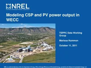
Modeling CSP and PV power output in WECC. TEPPC Data Working Group Marissa Hummon October 11, 2011. What is covered in this presentation?. Brief Overview of the S ub-Hour S ynthesis A lgorithm Classes of temporal variability Satellite data Class selection Modeled Plants

E N D
Modeling CSP and PV power output in WECC TEPPC Data Working Group Marissa Hummon October 11, 2011
What is covered in this presentation? • Brief Overview of the Sub-Hour Synthesis Algorithm • Classes of temporal variability • Satellite data Class selection • Modeled Plants • Filter for plant size • PV and CSP power output • Results & Analysis • Time series • Ramp distributions • Spatial – temporal correlations
Classes of temporal variability Class 0 is a special case of Class I
Site Clearness Index Analysis Spatial satellite data is used to calculate the relative proportions of cloud cover in an area for each hour. This data is related to the sub-hourly measurements of irradiance. These figures show five consecutive hours of aerial satellite data (left) and corresponding minutely ground-based irradiance data (right).
Area Filter • Reduction in variability as the irradiance signal is aggregated over an area. The larger the area, the lower the variability. Evidence: • Mills et al. demonstrated this: Southern Great Plains ARM Network • Marcos et al. demonstrated this: Spain • Perez et al. demonstrated this: California • Gueymard et al.: United States
Area Averaging A. Mills, R. Wiser, 2010, “Implications of Wide-Area Geographic Diversity for Short-Term Variability of Solar Power”, LBNL
Point source versus PV plant Milagro (0.52 km2) fc = 0.0032 Hz (5.2 min) Sesma (0.042 km2) fc = 0.0088 Hz (1.9 min)
Area Filter • PV plant footprint per PV capacity • Best Resource: 42 MW/km2 • Population PV: 38 MW/km2 • Rooftop: Capacity is evenly distributed over grid cell, 40-90 km2 • CSP plant footprint • 27.5 MW/km2 • Low pass filter (after Marcos et al.) • Cut-off frequency: fc = 0.0204 *sqrt(area) [hectares] • Range of plants affected: greater than 0.08 km2
PSDs (all classes) Synthetic (unfiltered) global horizontal Utility PV from 30 to 220 MW Distributed PV f [Hz]
Irradiance to Power Conversion • System Advisor Model: • PVWatts, a physical model of a “generic” silicon solar panel with inputs: • direct normal • diffuse horizontal • wind speed (ground) • temperature • Physical Trough Model for CSP • Select the “default” positions for most of the plant. It scales the plant with nominal capacity. • Storage: either 0 or 6 hours • Dry cooled plants • Solar Multiplier of 2 with storage
Analysis • Ramps (over all daylight hours) • Ramps with site aggregation • Site-to-site correlations
Regions of Sites for Ramp Correlations PV, best resource 1 CSP PV, population Rooftop 6 8 2 4 7 5 3
Power Ramps Group 3: Southern California
Ramp Correlations (2005)Area 2 Ramp correlations between sites a distance, d, apart, in a given region, follow this relationship, where t is duration of the ramp: c1 exp(-db1/t) + c2 exp(-db2/t) 1 6 8 2 4 7 5 3
Ramp Correlations (2005)Area 5 Ramp correlations between sites a distance, d, apart, in a given region, follow this relationship, where t is duration of the ramp: c1 exp(-db1/t) + c2 exp(-db2/t) 1 6 8 2 4 7 5 3
Ramp Correlations (2005)Area 7 Ramp correlations between sites a distance, d, apart, in a given region, follow this relationship, where t is duration of the ramp: c1 exp(-db1/t) + c2 exp(-db2/t) 1 6 8 2 4 7 5 3
Questions & Comments • Feel free to contact me at: • Marissa Hummon • National Renewable Energy Laboratory • Strategic Energy Analysis Center • 303-275-3269 • marissa.hummon@nrel.gov