Download
1 / 36
370 likes | 601 Views
Module 11: Experiments to study Variances-Variance Components Analysis and Nested Models.

E N D
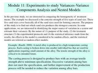
Module 11: Experiments to study Variances-Variance Components Analysis and Nested Models In the previous study, we are interested in comparing the homogeneity of treatment means. The example we discussed is the concrete strength of five types of sand size. These five sand sizes cover basically all of the sand sizes used for forming concrete. The purpose of the study is to find out which sand size produces the strongest concrete. In some applications, we are interested in identifying the major source of variation in a system and estimate their variances. By the nature of (1) purpose of the study, (2) the treatment structure (3) the experimental protocols and (4) the statistical inference made from the results, the effects in the model is considered to be random effects, and the statistical models are referred as random effect models. Example: (Kuehl, 2000): A metal alloy is produced in a high-temperature casting process. Each casting is broken down into smaller individual bas that are used for applications requiring small amount of the alloy. The tensile strength of the alloy is critical to its intended future. The casting process is designed to produce bars with an average tensile strength above minimum specifications. Excessive variation among bars does not meet the specification, and further improvement of the production process will be needed to reduce the variation among alloy bars.
Min m Min m • Through cause-effect analysis, two components contribute to the total variation in the tensile strength of bars are identified: • variability among fabrication casting, and • inconsistency within the casting process that affect bars from the same casting Purpose of the study: to quantify the uncertainty due to each component for further investigation of causes that result the uncertainty, and taking actions to reduce the uncertainty Experiment Design: Three fabrications casting in the same facility were randomly selected. Each casting was broken into individual bars. Ten randomly selected bars from each casting were tested . The interest is on identifying variations of tensile strength caused by casting in the facility and by bar within the casting, not about the mean differences among the tree casting.
The statistical model for identifying the two sources of variation for this random effects in this experiment is Row cast 1 cast 2 cast 3 1 88.0 85.9 94.2 2 88.0 88.6 91.5 3 94.8 90.0 92.0 4 90.0 87.1 96.5 5 93.0 85.6 95.6 6 89.0 86.0 93.8 7 86.0 91.0 92.5 8 92.9 89.6 93.2 9 89.0 93.0 96.2 10 93.0 87.5 92.5 The ANOVA table and expected mean squares for the random effect model:
Analyzing the Casting Process Data Row cast 1 cast 2 cast 3 1 88.0 85.9 94.2 2 88.0 88.6 91.5 3 94.8 90.0 92.0 4 90.0 87.1 96.5 5 93.0 85.6 95.6 6 89.0 86.0 93.8 7 86.0 91.0 92.5 8 92.9 89.6 93.2 9 89.0 93.0 96.2 10 93.0 87.5 92.5 Casting N Mean StDev cast 1 10 90.30 2.869 cast 2 10 88.43 2.456 cast 3 10 93.80 1.786
Factor Type Levels Values Casting random 3 cast 1 cast 2 cast 3 Analysis of Variance for Strength, using Adjusted SS for Tests Source DF Seq SS Adj SS Adj MS F P Casting 2 147.885 147.885 73.942 12.71 0.000 Error 27 157.102 157.102 5.819 Total 29 304.987 Expected Mean Squares, using Adjusted SS Source Expected Mean Square for Each Term 1 Casting (2) + 10.0000(1) 2 Error (2) Error Terms for Tests, using Adjusted SS Source Error DF Error MS Synthesis of Error MS 1 Casting 27.00 5.819 (2) Variance Components, using Adjusted SS Source Estimated Value Casting 6.812 Error 5.819 The EMS provides us information on how to conduct appropriate test. (2) Is the Random Error due Bars. se2 (1) Is variance due to Casting, sa2
Hands-on Activity • Find the estimate of the two variance components, and draw some suggestions for further investigation of reducing variations. • Compute a 95% confidence interval for component se2 • Compute a 90% confidence interval for component sa2 • Find the intra-class correlation and compute a 95% confidence interval for the intra-class correlation.
Sub-samples in Lab testing studies In many lab testing studies, a sample may be split into several sub-samples for testing. This sub-sampling introduces another source of random variation among sub-samples in addition to the source of random variations due to experimental units. It is necessary that the source of variation is identified in the study. Case Study: Pesticide Residue on Vegetables A concern is the pesticide residue remains on the plants after a time period. The residues are evaluated with chemical assays in the laboratory using plant samples from the field plots treated with the pesticide. Hypothesis of the Study: There are two standard chemical assays used to evaluate the residues. Which method can recover the pesticide residues better? Treatment Design: Two standard chemical methods A and B used on regular basis. Experimental Design: Six batches of plants, each batch from a single field plot, were sampled, and prepared for the residue analysis. Three batches were randomly assigned to each method in a completely randomized design setting. Within each batch prepared for testing, two sub-samples were taken for test. NOTE: The experimental unit for each method is batch. The testing unit is the sub-sample within each batch.
The statistical model that describes the experimental design with sub-sampling for this study is: Method Batch Sample Residue 1 1 1 120 1 1 2 110 1 2 3 120 1 2 4 100 1 3 5 140 1 3 6 130 2 4 7 71 2 4 8 71 2 5 9 70 2 5 10 76 2 6 11 63 2 6 12 68 Method N Mean StDev 1 6 120.00 14.14 2 6 69.83 4.26 (Data Source: Kuehl, 2000)
ANAOVA Table and the corresponding EMS Since there are two sources of variations contributed to the observations, the variance of Mean of each Method is NOTE: The model such as this is called a Mixed Model. It consists of both Fixed and Random effects components.
Estimating the variance components for the experiment with subsamples
Analysis of the Pesticide Residue Data Method N Mean StDev 1 6 120.00 14.14 2 6 69.83 4.26 Factor Type Levels Values Method fixed 2 1 2 Batch(Method) random 6 1 2 3 4 5 6 Analysis of Variance for Residue, using Adjusted SS for Tests Source DF Seq SS Adj SS Adj MS F P Method 1 7550.1 7550.1 7550.1 39.72 0.003 Batch(Method) 4 760.3 760.3 190.1 3.45 0.086 Error 6 330.5 330.5 55.1 (due to subsample) Total 11 8640.9
To test Method, use Source (2). To test Batch(method), use Source (3) Two variance components are: Expected Mean Squares, using Adjusted SS Source Expected Mean Square for Each Term 1 Method (3) + 2.0000(2) + Q[1] 2 Batch(Method) (3) + 2.0000(2) 3 Error (3) (due to subsample) Error Terms for Tests, using Adjusted SS Source Error DF Error MS Synthesis of Error MS 1 Method 4.00 190.1 (2) 2 Batch(Method) 6.00 55.1 (3) Variance Components, using Adjusted SS Source Estimated Value Batch(Method) 67.50 Error(due to Subsample) 55.08
Least Squares Means for Residue Method Mean 1 120.00 2 69.83 (Method)Batch 1 1 115.00 1 2 110.00 1 3 135.00 2 4 71.00 2 5 73.00 2 6 65.50 NOTE: The residual analysis reveals a serious violation of the constant variance assumption. What should be do?
Hands-On activity • Find appropriate transformation, conduct the data transformation, and reanalyzed the data. • Compare the results between the transformed data and the raw data. Do we notice any specific changes in our conclusion? • Obtain a 95% confidence interval for the mean of each chemical method using the raw data. • Obtain a 95% confidence interval for the mean difference between two chemical method using the raw data.
Nested Factor Experimental Designs and Mixed Factor Designs • In Inter-laboratory testing studies, this type of design occurs naturally. • Example: A study of a chromatographic method was condcuted for determining malathion. Ten labs participated in the study; each lab received a subsample of a technical grade malathion (Tech), two wettable powders (25% WP and 50% WP), and an emulsifiable concentrate (58% EC), and a dust. Each participant also received a internally tested standard of malathion (99.1%) along with the analytical method. (Wernimont, 1985). • Steps involving with this type of inter-lab study include at least: • Planning: Requirements for a protocol – objectives, analytical method, participating labs, preparation and distribution of of materials, replication scheme. • Executing: Specific rules and guidelines for participating labs, training of operators, analyzing material, recording and reporting the data. • 3. Screening data: Taking care of missing data, detecting biased labs, identifying outlying observations. Box-plots, h-plots, Youden’s plots, scatter plots are some common tools for screening. • 4. Analyzing data: Setting statistical models, using appropriate statistical methods, diagnosing assumptions, properly interpret the results. • 5. Preparing final report.
For the malathion testing study, one major purpose is to comparing the performance of lab performance using a variety of materials. One can also study the mean differences among materials and interaction between material and labs. • Different type of designs may be chosen. The simplest one for comparing the lab performance is a two variance component model for testing material. • Experimental design with two component model for testing a material: • Ten labs participated in the study. Each participated lab tested four samples of the same material. • The statistical model is
Raw Data for the Malathion Interlaboratory Study Row lab Rep WP25 WP50 1 1 1 26.17 50.76 2 1 2 26.22 50.67 3 1 3 25.85 50.81 4 1 4 25.80 50.72 5 2 1 26.44 50.82 6 2 2 26.57 50.90 7 2 3 25.80 51.04 8 2 4 26.06 50.96 9 3 1 26.95 52.53 10 3 2 26.91 52.54 11 3 3 26.98 52.55 12 3 4 26.91 52.47 13 5 1 26.23 50.20 14 5 2 26.00 50.47 15 5 3 26.22 50.39 16 5 4 26.18 50.43 17 6 1 25.45 51.65 18 6 2 25.62 51.67 Row lab Rep WP25 WP50 19 6 3 27.01 51.72 20 6 4 25.72 52.07 21 7 1 26.14 50.53 22 7 2 26.78 50.75 23 7 3 26.04 49.99 24 7 4 25.97 50.92 25 8 1 25.70 50.00 26 8 2 25.90 50.30 27 8 3 25.80 50.50 28 8 4 25.70 50.60 29 9 1 26.13 50.26 30 9 2 26.13 50.36 31 9 3 25.91 50.97 32 9 4 25.86 50.44 33 10 1 26.22 50.23 34 10 2 26.20 50.27 35 10 3 25.84 50.29 36 10 4 25.84 49.97
lab N Mean Median TrMean StDev 1 4 50.740 50.740 50.740 0.059 2 4 50.930 50.930 50.930 0.093 3 4 52.523 52.535 52.523 0.036 5 4 50.373 50.410 50.373 0.120 6 4 51.777 51.695 51.777 0.197 7 4 50.548 50.640 50.548 0.405 8 4 50.350 50.400 50.350 0.265 9 4 50.508 50.400 50.508 0.317 10 4 50.190 50.250 50.190 0.149
Analysis of Variance for WP50%_1 Source DF SS MS F P laborato 8 19.1570 2.3946 50.958 0.000 Error 27 1.2688 0.0470 Total 35 20.4258 Variance Components Source Var Comp. % of Total StDev laborato 0.587 92.59 0.766 Error 0.047 7.41 0.217 Total 0.634 0.796 Expected Mean Squares 1 laborato 1.00(2) + 4.00(1) 2 Error 1.00(2) It is clearly indicates that 92.6% of the total variance of each observation is the between-lab. That is the lab averages are very different. This was also shown by the X-bar chart. This makes sense , since operators will be familiar with the lab facilities. A further action is to
Bonferroni confidence intervals for standard deviations Lower Sigma Upper N Factor Levels 0.027423 0.059442 0.46874 4 1 0.042948 0.093095 0.73412 4 2 0.016580 0.035940 0.28341 4 3 0.055152 0.119548 0.94272 4 5 0.090980 0.197210 1.55514 4 6 0.186613 0.404506 3.18983 4 7 0.122058 0.264575 2.08637 4 8 0.146246 0.317004 2.49981 4 9 0.068634 0.148773 1.17318 4 10
Quantify the uncertainty of Individual Lab Mean and determine a 95% confidence interval for the lab mean. The ANOVA technique assumes constant variance, therefore, there is a common variance component for each Lab mean Hence, the estimate from the data is: =.047/4 = .012 95% CI for Lab 1 is
Hands-on Activity • Conduct the same analysis for the PW25% variable: • Set up a statistical model for this experiment. • Descriptive summary with dot-plots Vs Labs. • Testing constant variance, and find Bonferroni confidence interval of within-lab s.d.. • Conduct Xbar, R-charts analysis. • Conduct ANOVA and estimate variance components. • Find variance of lab mean and obtain a 95% CI for the Lab Mean of Lab 3.
2. Experimental design with three variance components In the two-component model, we assume that the testing processes are similar day in and day out. However, in some situations, lab testing may not be consistent day in and day out. A three variance component design may be implemented if there is a doubt about the consistency from day to day. A participated lab tested four samples of the material per day, and will be asked to conduct the same test at three randomly chosen days, not known to the participated lab. A statistical model based on this design is :
A general setting of a design with three nested factors The Inter-laboratory testing study is one case example of the nested design. For a general three nest factors, the effects can be mixed with fixed and random, depending on the actual experiment. The following is the corresponding statistical model for three nested factors. NOTE: It is difficult to estimate the components or conduct proper F-tests for each factor when the model is mixed and complicated. Fortunately, Minitab can provide the EMS and show how the F-tests are conducted in ANOVA table.
ANOVA Table and the EMS for the Three Nested Random Factor Experiment
A Case Study of Three Nested Random Factor Experiment A laboratory performs serum assays critical for correct medical diagnosis. It is important to maintain program to monitor the performance of assays and ensure accurate information for diagnosis. The important sources of variation in the assays are days on which the assays are conducted, the replicate runs within days, and the replicate serum sample preparations within runs. The quality control program requires that a spectrophotometer be tested within several runs on each of several days with serum standards used in the laboratory for control runs. Replicate serum preparations are evaluated within each of the runs. The data in the following table are observations from a design for the analysis of glucose standards. There are three (c=3) replications of the standard prepared for each of two runs(b=2) on each of three days (a=3).
Row Day Run Sample glucose 1 1 1 1 42.5 2 1 1 2 43.3 3 1 1 3 42.9 4 1 2 1 42.2 5 1 2 2 41.4 6 1 2 3 41.8 7 2 3 1 48.0 8 2 3 2 44.6 9 2 3 3 43.7 10 2 4 1 42.0 11 2 4 2 42.8 12 2 4 3 42.8 13 3 5 1 41.7 14 3 5 2 43.4 15 3 5 3 42.5 16 3 6 1 40.6 17 3 6 2 41.8 18 3 6 3 41.8 Three factors: Day,Run within Day and Replicates within Run are all random effect factors. Bonferroni confidence intervals for standard deviations Lower Sigma Upper N Run Day 0.170862 0.40000 6.1903 3 1 1 0.170862 0.40000 6.1903 3 2 1 0.968739 2.26789 35.0974 3 3 2 0.197294 0.46188 7.1480 3 4 2 0.363290 0.85049 13.1620 3 5 3 0.295941 0.69282 10.7219 3 6 3 On Day2, the three replications for run 3 are very different, especially the one with glucose = 48. A close check is needed. In this analysis,we assume there was no special causes for this data. (Data from Kuehl, 2000. Unit: mg/dl)
Factor Type Levels Values Day random 3 1 2 3 Run(Day) random 6 1 2 3 4 5 6 Analysis of Variance for glucose, using Adjusted SS for Tests Source DF Seq SS Adj SS Adj MS F P Day 2 13.763 13.763 6.882 1.26 0.400 Run(Day) 3 16.357 16.357 5.452 4.75 0.021 Error 12 13.760 13.760 1.147 Total 17 43.880 Unusual Observations for glucose Obs glucose Fit SE Fit Residual St Resid 7 48.0000 45.4333 0.6182 2.5667 2.94R R denotes an observation with a large standardized residual. • The analysis indicates there is no significant day-to-day variation. But there is a significant variation among the runs within Day. • The 1st replicate of the 3rd run (on 2nd day) is an unusual case.
Source Expected Mean Square for Each Term 1 Day (3) + 3.0000(2) + 6.0000(1) 2 Run(Day) (3) + 3.0000(2) 3 Error (3) Error Terms for Tests, using Adjusted SS Source Error DF Error MS Synthesis of Error MS 1 Day 3.00 5.452 (2) 2 Run(Day) 12.00 1.147 (3) Variance Components, using Adjusted SS Source Estimated Value Day 0.2382 Run(Day) 1.4352 Error 1.1467 The error term of the F-test for testing the significance of sa2is Run(Day). The error term for testing Run(Day) is ‘Error’. Three variance components are The variance component for Day is non-significant. Run(day) and random error due to replications within Run are similar.
Least Squares Means for glucose Day Mean 1 42.35 2 43.98 3 41.97 (Day)Run 1 1 42.90 1 2 41.80 2 3 45.43 2 4 42.53 3 5 42.53 3 6 41.40 The standard error for the grand mean and the mean of ith level of factor A, are: 100(1-a)% confidence interval for mean of the ith level of factor A:
Hands-on Activity • Obtain each variance component by hand. • Obtain the estimate of variance of grand mean glucose and a day mean glucose. • Obtain a 95% confidence interval of the grand mean glucose and a day mean glucose. • Compute the proportion of each variance component. • Exclude the case (7), value = 48, and re-analyze the data.