Download
1 / 42
420 likes | 546 Views
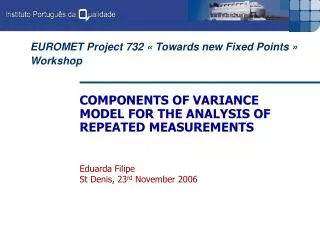
EUROMET Project 732 « Towards new Fixed Points » Workshop. COMPONENTS OF VARIANCE MODEL FOR THE ANALYSIS OF REPEATED MEASUREMENTS Eduarda Filipe St Denis, 23 rd November 2006. Summary. Introduction General principles and concepts The Nested or Hierarchical Design

E N D
EUROMET Project 732 « Towards new Fixed Points »Workshop COMPONENTS OF VARIANCE MODEL FOR THE ANALYSIS OF REPEATED MEASUREMENTS Eduarda Filipe St Denis, 23rd November2006
Summary • Introduction • General principles and concepts • The Nested or Hierarchical Design • Application example of a three-stage nested experiment.
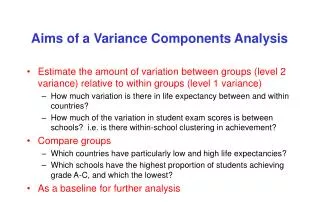
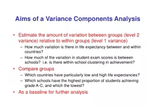
Introduction • The realization of the International Temperature Scale of 1990 - ITS90 requires that the Laboratories usually have more than one cell for each fixed point. • The Laboratory may consider one of the cells as a reference cell and its reference value, performing the other(s) the role of working standard(s), or the Laboratory considers its own reference value as the average of the cells.
Introduction • In both cases, the cells must be regularly compared and the calculation of the uncertainty of these comparisons performed. • A similar situation exists when the laboratory compares its own reference value with the value of a travelling standard during an inter-laboratory comparison.
Introduction • These comparisons experiments are usually performed with two or three thermometers to obtain the differences between the cells. • The repeatability measurements are performed each day at the equilibrium plateau and the experiment is repeated in subsequent days. This complete procedure may also be repeated some time after.
Introduction • The uncertainty calculation should take into account these time-dependent sources of variability, arising fromshort-term repeatability, the day-to-day or ”medium term” reproducibility and thelong-term random variations in the results;
Introduction • The Type A method of evaluation by the statistical analysis of the data obtained from the experimentis performedusing theAnalysis of Variance (ANOVA)for designs, consisting ofnested or hierarchical sequencesof measurements.
ANOVA definition ISO 3534-3, Statistics – Vocabulary and Symbols “Technique, which subdivides the total variation of a response variable into meaningful components, associated with specific sources of variation”.
General principles and concepts • Experimental design is a statistical tool concerned with planning the experiments to obtain the maximum amount of information from the available resources • This tool is used generally for the improvement and optimisation of processes
General principles and concepts • it can be used to test the homogeneity of a sample(s) • to identify the results that can be considered as “outliers” • to evaluate the components of variance between the “controllable” factors
General principles and concepts • tool applied to Metrology for the analysis of large amount of repeated measurements • Measurements in: • short-term repeatability • day-to-day reproducibility • long-term reproducibility • permitting “mining” the results and to include this “time-dependent sources of variability” information at the uncertainty calculation.
General principles and concepts • In the comparison experiment to be described, the factors are the standard thermometers, the subsequent days measurements and the run measurements. • These factors are considered as random samples of the population from which we are interested to draw conclusions.
The nested or hierarchical design. DefinitionISO 3534-3, Statistics – Vocabulary and Symbols “The experimental design in which each level of a given factor appears in only a single level of any other factor”. Purpose of this model To deduce the values of component variances that cannot be measured directly.
The nested or hierarchical design. General model • The factors are hierarchized like a “tree” and any path from the “trunk” to the “extreme branches” will find the same number of nodes. The analysis of each factor is done with: “Random Effects One-way ANOVA” or components-of-variance model, nested in the subsequent factor.
1 1 1 1 1 1 1 1 A A B B 1 2 1 2 Measurements M = 2 Factor T T = 2 D = 10 Factor D 1 2 P = 2 Factor P Observer Nested design
The nested or hierarchical design. General model For one factor with a different levels taken randomly from a large population, where Miis the expected (random) value of the group of observations i, mthe overall mean, tithe i th group random effect and eijthe random error component.
The nested or hierarchical design. General model • For the hypothesis testing, the errors and the factor-levels effects are assumed to be normally and independently distributed, respectively eij~ N (0,s2) and ti ~ N (0,st2). • The variance of any observation y is composed by the sum of the variance components
The nested or hierarchical design. General model • The test is unilateral and the hypotheses are: • That is, if the null hypothesis is true, all factor-effects are “equal” and each observation is made up of the overall mean plus the random error eij ~ N (0,s2).
SSFactor SSE = 0 SSFactor sum of squares of differences between factor-level averages and the grand average ora measure of the differences between factor-level SSE a sum of squares of the differences of observations within a factor-level from the factor-level average, due to the random error The nested or hierarchical design. General model The total sum of squares (SST), a measure of total variability in the data, may be expressed by:
The nested or hierarchical design. General model Dividing each sum of squares by the respectively degrees of freedom, we obtain the corresponding mean squares (MS): • MSFactor - mean square between factor-level is: • an unbiased estimate of the variances 2, ifH0 is true • or a surestimate of s 2, if H0 is false. • MSError - mean square within factor (error) is always • the unbiased estimate of the variance s 2.
Fis theFisher samplingdistribution with aand a x (n -1) degrees of freedom The nested or hierarchical design. General model To test the hypotheses, we use the statistic: If F0 > Fa, a-1, a(n-1) , we reject the null hypothesis. and conclude that the variance s2is significantly different of zero.
The nested or hierarchical design. General model The expected value of the MSFactoris: and the variance component of the factor is obtained by:
The nested or hierarchical design. General model Considering now the three level nested design of the figure the mathematical model is: yrdtm(rdtm) th observation moverall mean PrP th random level effect DdD th random level effect TtT th random level effect ertdm random error component.
The nested or hierarchical design. General model The errors and the level effects are assumed to be normally and independently distributed, respectively with mean zero and variance s2and with mean zero and variances sr2,sd2 andst2. The variance of any observation is composed by the sum of the variance components and the total number of measurements N is obtained by the product of the dimensions N = P × D × T × M.
The nested or hierarchical design. General model The total variability of the data can be expressed by
The nested or hierarchical design. General model • Dividing by the respective degrees of freedom • P –1 P (D -1)P D (T -1) P D T (M -1) • Equating the mean squares to their expected values • Solving the resulting equations • We obtain the estimates of the components of the variance.
A – water vapour B – water in the liquid phase C – Ice mantle D – thermometer (SPRT) well t = 0,01 ºC Example of the comparison of two thermometric Water triple point cells in a three-stage nested experiment Two water cells, JA and HS Two standard platinum resistance thermometers (SPRTs) A and B.
Four measurement differences obtained daily with the two SPRTs • This set of measurements repeated during ten consecutive days. • And two weeks after a complete run was repeated Run 2/Plateau 2.
Example of the comparison of two thermometric Water triple point cells in a three-stage nested experiment • In this nested experiment, are considered the effects of: • Factor‑P from the Plateaus (P = 2) • Factor-D from the Days (D = 10) for the same Plateau • Factor-T from the Thermometers (T = 2) for the same Day and for the same Run • the variation between Measurements (M = 2) for the same Thermometer, the same Day and for the same Plateau or the residual variation.
Example of the comparison of two thermometric Water triple point cells in a three-stage nested experiment
Example of the comparison of two thermometric Water triple point cells in a three-stage nested experiment Schematic representation of the observed temperatures differences
Example of the comparison of two thermometric Water triple point cells in a three-stage nested experiment Analysis of variance table F0 values compared with the critical values Fn1,n2 (a = 5%) F0,05, 1, 18 = 4,4139 for the Plateau/Run effect F0,05, 18,20 = 2,1515 for the Days effect and F0,05, 20, 40 =1,8389 for the Thermometers effect.
Example of the comparison of two thermometric Water triple point cells in a three-stage nested experiment • F0 values are inferior to the F distribution for the factor-days and factor-thermometers so the null hypotheses are not rejected. • At the Plateau factor, the null hypothesis is rejected for a = 5% so a significant difference exists between the two Plateaus
Example of the comparison of two thermometric Water triple point cells in a three-stage nested experiment • equating the mean squares to their expected values • we can calculate the variance components • and • include them in the budget of the components of uncertainty
Example of the comparison of two thermometric Water triple point cells in a three-level nested experiment Uncertainty budget for components of uncertainty evaluated by a Type A method
Example of the comparison of two thermometric Water triple point cells in a three-level nested experiment • These components of uncertainty, evaluated by Type A method, reflect the random components of variance due to the factors effects • This model for uncertainty evaluation that takes into account the time-dependent sources of variability it is foreseen by the GUM
Example of the comparison of two thermometric Water triple point cells in a three-level nested experiment Comparison of different approaches • Components of uncertainty evaluated by a Type A method • Nested structure: uA= 20,5 mK • Standard deviation of the mean of 80 measurements uA= 2,2 mK • Standard deviation of the mean 1st Plateau (40 measurements) uA= 2,8 mK(the 2nd plateau considered as reproducibility and evaluated by a type B method)
Concluding Remarks • The plateaus values continuously taken where previously analyzed in terms of its normality. • The nested-hierarchical design was described as a tool to identify and evaluate components of uncertainty arising from random effects. • Applied to measurement, it is suitable to calculate the components evaluated by a Type A method standard uncertainty in time-dependent situations.
Concluding Remarks • An application of the design has been used to illustrate the variance components analysis in a three-factor nested model of a short, medium and long-term comparison of two thermometric fixed points. • The same model can be applied to other staged designs, easily treated in an Excel spreadsheet.
REFERENCES • BIPM et al, Guide to the Expression of Uncertainty in Measurement (GUM), 2nd ed., International Organization for Standardization, Genève, 1995, pp 11, 83-87. • ISO 3534-3, Statistics – Vocabulary and Symbols – Part 3: Design of Experiments, 2nd ed., Genève, International Organization for Standardization, 1999, pp. 31 (2.6) and 40-42 (3.4) • Milliken, G.A., Johnson D. E., Analysis of Messy Data. Vol. I: Designed Experiments. 1st ed., London, Chapmann & Hall, 1997. • Montgomery, D., Introduction to Statistical Quality Control, 3rd ed., New York, John Wiley & Sons, 1996, pp. 496-499. • ISO TS 21749 Measurement uncertainty for metrological applications — Simple replication and nested experiments Genève, International Organization for Standardization, 2005. • Guimarães R.C., Cabral J.S., Estatística, 1st ed., Amadora: Mc-Graw Hill de Portugal, 1999, pp. 444-480. • Murteira, B., Probabilidades e Estatística. Vol. II, 2nd ed., Amadora, Mc-Graw Hill de Portugal, 1990, pp. 361-364. • Box, G.E.P., Hunter, W.G., Hunter J.S., Statistics for Experimenters. An Introduction to Design, Data Analysis and Model Building, 1st ed., New York, John Wiley & Sons, 1978, pp. 571-582. • Poirier J., “Analyse de la Variance et de la Régression. Plans d’Experience”, Techniques de l’Ingenieur, R1, 1993, pp. R260-1 to R260-23.