Download
1 / 17
170 likes | 334 Views
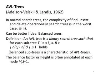
AVL-Trees (Adelson-Velskii & Landis, 1962). In normal search trees, the complexity of find, insert and delete operations in search trees is in the worst case: (n). Can be better! Idea: Balanced trees.

E N D
AVL-Trees (Adelson-Velskii & Landis, 1962) In normal search trees, the complexity of find, insert and delete operations in search trees is in the worst case: (n). Can be better! Idea: Balanced trees. Definition: An AVL-tree is a binary search tree such that for each sub-tree T ' = < L, x, R >| h(L) - h(R) | 1 holds (balanced sub-trees is a characteristic of AVL-trees). The balance factor or height is often annotated at each node h(.)+1.
|Height(I) – hight(D)| < = 1 Thisisan AVL tree
Thisis NOT an AVL tree (node * doesnotholdtherequiredcondition)
Goals 1. How can the AVL-characteristics be kept when inserting and deleting nodes? 2. We will see that for AVL-trees the complexity of the operations is in the worst case = O(height of the AVL-tree) = O(log n)
Preservation of the AVL-characteristics After inserting and deleting nodes from a tree we must procure that new tree preserves the characteristics of an AVL-tree: Re-balancing. How ?: simple and double rotations
Only 2 cases (an their mirrors) • Let’s analyze the case of insertion • The new element is inserted at the right (left) sub-tree of the right (left) child which was already higher than the left (right) sub-tree by 1 • The new element is inserted at the left (right) sub-tree of the right (left) child which was already higher than the left (right) sub-tree by 1
Rotation (for the case when the right sub-tree grows too high after an insertion) Istransformedinto
Double rotation (for the case that the right sub-tree grows too high after an insertion at its left sub-tree) Double rotation Istransformedinto
b First rotation a c W x y Z new a Second rotation b W c x new y Z
Re-balancing after insertion: After an insertion the tree might be still balanced or: theorem: After an insertion we need only one rotation of double-rotation at the first node that got unbalanced * in order to re-establish the balance properties of the AVL tree. (* : on the way from the inserted node to the root). Because: after a rotation or double rotation the resulting tree will have the original size of the tree!
The same applies for deleting • Only 2 cases (an their mirrors) • The element is deleted at the right (left) sub-tree of which was already smaller than the left (right) sub-tree by 1 • The new element is inserted at the left (right) sub-tree of the right (left) child which was already higher that the left (right) sub-tree by 1
The cases Deleted node 1 1 1
Re-balancing after deleting: After deleting a node the tree might be still balanced or: Theorem: after deleting we can restore the AVL balance properties of the sub-tree having as root the first* node that got unbalanced with just only one simple rotation or a double rotation. (* : on the way from the deleted note to the root). However: the height of the resulting sub-tree might be shortened by 1, this means more rotations might be (recursively) necessary at the parent nodes, which can affect up to the root of the entire tree.
About Implementation • While searching for unbalanced sub-tree after an operation it is only necessary to check the parent´s sub-tree only when the son´s sub-tree has changed it height. • In order make the checking for unbalanced sub-trees more efficient, it is recommended to put some more information on the nodes, for example: the height of the sub-tree or the balance factor (height(left sub-tree) – height(right sub-tree)) This information must be updated after each operation • It is necessary to have an operation that returns the parent of a certain node (for example, by adding a pointer to the parent).
Complexity analysis– worst case Be h the height of the AVL-tree. Searching: as in the normal binary search tree O(h). Insert: the insertion is the same as the binary search tree (O(h)) but we must add the cost of one simple or double rotation, which is constant : also O(h). delete: delete as in the binary search tree(O(h)) but we must add the cost of (possibly) one rotation at each node on the way from the deleted node to the root, which is at most the height of the tree: O(h). All operations are O(h).
Calculating the height of an AVL tree Principle of construction Be N(h) the minimal number of nodes In an AVL-tree having height h. N(0)=1, N(1)=2, N(h) = 1 + N(h-1) + N(h-2) für h 2. N(3)=4, N(4)=7 remember: Fibonacci-numbers fibo(0)=0, fibo(1)=1, fibo(n) = fibo(n-1) + fibo(n-2) fib(3)=1, fib(4)=2, fib(5)=3, fib(6)=5, fib(7)=8 By calculating we can state: N(h) = fibo(h+3) - 1 0 1 2 3
Be n the number of nodes of an AVL-tree of height h. Then it holds that: n N(h) , By making p = (1 + sqrt(5))/2 und q = (1- sqrt(5))/2 we can now write n fibo(h+3)-1 = ( ph+3 – qh+3 ) / sqrt(5) – 1 ( p h+3/sqrt(5)) – 3/2, thus h+3+logp(1/sqrt(5)) logp(n+3/2), thus there is a constant c with h logp(n) + c = logp(2) • log2(n) + c = 1.44… • log2(n) + c = O(log n).