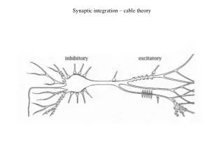
Synaptic integration – cable theory
Synaptic integration – cable theory. Isopotential sphere. Current injected into a spherical cell will distribute uniformly across the surface of the sphere. The current flowing across a unit area of the membrane:. For a finite step of current:.

Synaptic integration – cable theory
E N D
Presentation Transcript
Isopotential sphere Current injected into a spherical cell will distribute uniformly across the surface of the sphere. The current flowing across a unit area of the membrane: For a finite step of current: For a sphere, a relationship between Im and I0 is: where The input resistance: - time constant After the current step: The input resistance of a sphere: For long impulse Im(t -> inf) - stan ustalony
Nonisopotential cell (cylinder) Assumptions: 1.Uniform membrane. Membrane parameters are constant and they are not dependent on the membrane potential. 2.The current flows along dimension x, radial current is zero. 3. Extracellular resistance, r0, is 0. Recalling We obtain the cable equation Vm is function of time and distance from the site of injection. The decrease in Vm with distance is given by Ohm’s law: The decrease in ii with distance is equal to the current that flows across the membrane: In another form: We obtain: • space or length constant
The cable equation Let: The cable equation becomes: We will be using solutions to this equation to derrive equations that describe a number of specific situations like inifite cable, finite cable, and finite cable with lumped soma.
Solutions of the cable equations – infinite cable We will consider solution to the cable equation for a situation where a step current is injected into an infinitely long cable A general solution to the cable equation is erfc(x) – complementary error function
Solutions of the cable equations – infinite cableSteady – state solution We are seeking steady – state solution Interpretaton of l: l reflects steady – state properties of the cable. It is the distance at which potential has decayed to 1/e of the value at x = 0. or The input resistance - infinite cable The input resistance – semi-infinite cable
Solutions of the cable equations – infinite cableTransient solution Transient solution at x,X = 0 Infinite cable Semi-infinite cable
Transient solution and estimation of the membrane time constant Transient solution at x,X = 0 Transient solution for isopotential sphere Membrane time constant The membrane potential of the infinite cable changes faster toward its steady-state value than that of the ispotential sphere. This was extremly important result of Rall’s work. It demonstrated why early estimates of membrane time constants from neurons were too low. The response to current step (charging curve) was assumed to be single exponential end the membrane time constant was estimated from the time to reach 63% of the steady-state value. Using point 0.63 on the error function gives estimate 0.4, instead of (correct value) 1.
Solutions of the cable equations – infinite cableFull solution • Observations: • At large t, the distribution of potential along the cable is the steady – state solution. • At intermediate values of t, the decay of potential with distance along the cable is greater than at the steady-state. • At x = 0 the charging curve is described by erfc(T1/2). • At values of x increasing from 0, the charging curves show slower rising phases and reach a smaller steady-state value. Solution of the cable equation as a function of time and distance for a step of current injected at x = 0 into a semi-finite cable.
Solutions of the cable equations – finite cableSteady – state solution I0 The cable equation: x = 0 x = l Under steady – state conditions We will consider two boundary conditions for x = l - sealed end - open end The cable equation can be reduced to: We introduce new variables: • electrotonic distance • electrotonic length A general solution: Hiperbolic cosine and sine:
Solutions of the cable equations – finite cableSteady – state solution The general solution of the cable equation can be rewritten using the hyperbolic functions as: or at X = L, Let BL = C2/VL and substitute it back into the equation. BLis the boundary condition for different end terminations At X = 0: or Substitute this back into the equation, we obtain
finite cable with sealed end finite cable with open end semi-infinite cabl. Solutions of the cable equations – finite cableSteady – state solution, boundary conditions the steady state solution of the cable equation for a finite-length cable. Effects of the boundary conditions - conductance of a semi-infinite cable - conductance of the terminal membrane than 1. If that is the same as for a semi-infinite cable that is 2. If (sealed end) that is 3. If (open end) Comparison of voltage decays along finite cables of different electrotonic lenghts and with different terminations. Current injected at x = 0.
Solutions of the cable equations – finite cableTransient solution The complete solution of the cable equation can be written as: where The first term of the equation: Corresponds to membrane time constant if the cable has uniform membrane properties Charging curves for finite cables of different electrotonic lenghts. A step curent is injected and the voltage is measured at x = 0.
Solutions of the cable equations – finite cable– AC current The steady-state decay of potential along a cable is much greater if the applied current changes in time. The AC length constant depends on DC length constant and frequency as follows: f – frequency (in Hz) Voltage attenuation along a finite cable (L = 1) for current injections DC to 100 Hz at X = 0 (soma)
Rall model for neurons Now, we can use the decriptions for the semi-infinite and finite-length cables to derrive Rall model of a neuron. This model provides a theoretical support for unerstanding the spread of current and voltage in complicated dendritic trees. • Assumptions: • Uniform membrane properties Ri, Rm, Cm • R0= 0 • Soma represented as an isopotential sphere • All dendrited terminated at the same electrotonic length.
Rall model for neurons Schematic diagram of a neuron with a branched dendritic tree. X1, X2, X3 are three representative branch points, d – is the diameter of the respective branches. Final branches are assumed to extend to infinity and thus are semi-infinite cables. Let’s recall the input resistance of semi-infinite cable
Rall model for neurons Input resistance of semi-infinite cable Input conductance of the semi-infinite cable Total conductance is sum of all parallel conductances, hence a total input conductance at X3 is This can be simplified If instead of a branch point at X3 , cable d211 was extended to infinity and detached at the same spot, its input conductane would be: Input conductance of the cable d3111 Rall recognized that if A similar equation exists for cable d3112 than having branch point X3 with branches d3111 and d3112 is exactly equivalent to extending branch d211 to infinity!
Rall model for neurons If we had done the same operation at the branch point along d212, then at X2 there would be two semi-infinite cables d211 i d212 attached to branch d11. As before, if Applying 3/2 power rule: then which is equivalent to extending cable d11 to infinity. one can reduce the entire dendritic tree to an equivalent semi-infinite cylinder. A number of studies has suggested that the branching in dendrites o spinal motor neurons, cortical neurons and hippocampal neurons closely approximates the 3/2 power rule.
Rall model for neuronsEquivalent finite cylinder Dendrites are usually better represented by finite-length cables, because usually l < 2l. The equation for the input conductance of finite cable is: and is also proportional to d3/2. L – electrotonic length, assumed to be the same for all dendrites. Using the relations: We obtain Applying the equations for input conductance, the 3/2 power rule and assumption of the same L for all dendrites one can reduce any dendritic tree to a single equivalent cylinder of diameter d0 electrotonic length L. Furthermore recalling that, L = l/l, for such a tree:
Rall model for neurons – application to synaptic inputs The main reason for studying the electrotonic properties of neurons is to help to understand the function of dendritic synaptic inputs. Using his theory, Rall demonstrated that distal synaptic inputs produce measurable signal at the soma. He estimated that the electrotonic length o spinal motor neurons was about 1.5. He calculated the changes in membrane potential measured in the soma in response to brief current steps to the soma, middle region of the dendrites and distal dendrites. • Results: • the amplitude of synaptic potential measured at soma is attenuted with input distance from the soma • the rise time and peak amplitude of the inputs is slowed and delayed for more distant inputs • the decay time of all inputs is the same (this is because the potential due to synaptic input cannot decay slower than the membrane time constant).
Functional properties of the synapses Synapses don’t inject step current, they produce brief conductance change often approximated by an alpha function gs = Gs(t/α)e-αt. Synaptic conductance gs and excitatory postsynaptic potential EPSP. If the time course of gs is briefcompared to tm, EPSP will decay with the membrane time constant. Synapse A Rising time constant Cm/(GsA + Gr) Decay time constant Cm/ Gr Synapse A + B Rising time constant Cm/(GsA + GsA + Gr) Decay time constant Cm/ Gr Parralel conductance model representing the separate synaptic inputs, A and B.
Dendritic computations – an example Summation of dendritic inputs in a model neuron. When four synaptic inputs (A–D) arrive at four separate locations of a neuron with brief intervals, spatial summation can be significant only when they synapses are activated in a preffered order i.e., D to A, but not A to D. From Arbib,M. A., 1989, The Metaphorical Brain 2:NeuralNetworks and Beyond, New York:Wiley-Interscience, p. 60. Livingstone MS.Mechanisms of direction selectivity in macaque V1. Neuron. 1998, 20(3):509-26.
Cable and compartmental models of dendritic trees Various dendritic trees (a, b, c) and their computer models (d, e). Dendrites are modeled either as a set of cylindrical membrane cables (B) or as a set of discrete isopotential RC compartments (C). B. In the cable representation, the voltage can be computed at any point in the tree by using the continuous cable equation and the appropriate boundary conditions imposed by the tree. An analytical solution can be obtained for any current input in passive trees of arbitrary complexity with known dimensions and known specific membrane resistance and capacitance (RM,CM) and specific cytoplasm (axial) resistance (RA). C. In the compartmental representation, the tree is discretized into set of interconnected RC compartments. Each is a lumped representation of the membrane properties of a sufficiently small dendritic segment. Compartments are connected via axial cytoplasmic resistances. In this approach, the voltage can be computed at each compartment for any(nonlinear) input and for voltage and time-dependent membrane properties (not only passive membranes).
Dendirtic computations - summary From Idan Segev and Michael LondonDendritic Processing. In M. Arbib (editor). The Handbook ofBrain Theoryand Neural Networks. THE MIT PRESSCambridge,MassachusettsLondon, England, 2002
Dendritic computations - logical operations Własności dendrytów umożliwają wykonywanie operacji logicznych. Z Idan Segev and Michael LondonDendritic Processing. Rozdział w M. Arbib (edytor). The Handbook ofBrain Theoryand Neural Networks. THE MIT PRESSCambridge,MassachusettsLondon, England, 2002
Dendritic computations - coincidence detection In birds, a special type of neuron is responsible for computing the time difference between sounds arriving to the two ears. Coincident inputs from both ears arriving to the two dendrites are summed up at the soma and cause the neuron to emit action potentials. However, when coincident spikes arrive from the same ear, they arrive at the same dendrite and thus their summation is sublinear, resulting in a subthreshold response. In layer 5 pyramidal neurons excitatory distal synaptic input (EPSP) that coincides with backpropagation of the action potential (bAP) results in a large dendritic Ca 2+ spike, which drives a burst of spikes in the axon. Otherwise, a single AP is generated. From: Michael London and Michael Hausser. Dendritic Computation. Annu. Rev. Neurosci.2005. 28:503–32
Dendritic computations - feature extraction Mapping of synaptic inputs onto dendritic branches may play a role in feature extraction responsible for face recognition. In neurons with active dendrites, clusters of inputs active synchronously on the same branch can evoke a local dendritic spike, which leads to significant amplification of the input. Specific configuration of inputs may trigger a spike while activation of synapses at different branches will not generate a response. The features extracted by dendrites may be fed into a soma or features extracted by multiple neurons are fed to a next cortical cell. From: Michael London and Michael Hausser. Dendritic Computation. Annu. Rev. Neurosci.2005. 28:503–32
Encoding/decoding information in a neuron Exploring dendritic input-output relation using information theory. (A) Reduced model of a neuron consisting of a passive dendritic cylinder, a soma and an excitable axon. The dendritic cylinder is bombarded by spontaneous background synaptic activity (400 excitatory synapses, each activated 10 times/s; 100 inhibitory synapses, each activated 65 times/s). (B) Soma EPSPs for a proximal (red line) and a distal (blue line) synapse. (C) Two sample traces of the output spike train measured in the modeled axon. Identical background activity was used in both cases; the location of only one excitatory synapse was displaced from proximal to distal. This displacement noticeably changes the output spike train. (D) The mutual information (MI), which measures how much could be known about the input (the presynaptic spike train) by observing the axonal output, is plotted as a function of the maximal synaptic conductance. The distal synapse transmits significantly less information compared to the proximal synapse. For strong proximal synapses, the MI is saturated because, for large conductance values, each input spike generates a time-locked output spike and no additional information is gained by further potentiating this synapse. From: Idan Segev and Michael London. Untangling Dendrites with Quantitative Models. Science 290, 2000