Download
1 / 13
130 likes | 268 Views
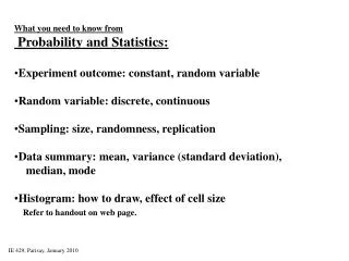
What you need to know from Probability and Statistics: Experiment outcome: constant, random variable Random variable: discrete, continuous Sampling: size, randomness, replication Data summary: mean, variance (standard deviation), median, mode Histogram: how to draw, effect of cell size

E N D
What you need to know from • Probability and Statistics: • Experiment outcome: constant, random variable • Random variable: discrete, continuous • Sampling: size, randomness, replication • Data summary: mean, variance (standard deviation), • median, mode • Histogram: how to draw, effect of cell size • Refer to handout on web page. IE 429, Parisay, January 2010
What you need to know from • Probability and Statistics (cont): • Probability distribution: how to draw, mass function, • density function • Relationship of histogram and probability distribution • Cumulative probability function: discrete and continuous • Standard distributions: parameters, other specifications • Read Appendix C and D of your textbook. IE 429, Parisay, January 2010
Relation betweenExponential distribution ↔ Poisson distribution Xi : Continuous random variable, time between arrivals, has Exponential distribution with mean = 1/4 X1=1/4 X2=1/2 X3=1/4 X4=1/8 X5=1/8 X6=1/2 X7=1/4 X8=1/4 X9=1/8 X10=1/8 X11=3/8 X12=1/8 0 1:00 2:00 3:00 Y1=3 Y2=4 Y3=5 Yi : Discrete random variable, number of arrivals per unit of time, has Poisson distribution with mean = 4. (rate=4) Y ~ Poisson (4) IE 429, Parisay, January 2010
What you need to know from • Probability and Statistics (cont): • Confidence level, significance level, confidence interval, half width • Goodness-of-fit test • Refer to handout on web page. IE 429, Parisay, January 2010
Demo on Queuing Concepts Refer to handout on web page. Basic queuing system: Customers arrive to a bank, they will wait if the teller is busy, then are served and leave. Scenario 1: Constant interarrival time and service time Scenario 2: Variable interarrival time and service time Objective: To understand concept of average waiting time, average number in line, utilization, and the effect of variability. IE 429, Parisay, January 2010
Scenario 1: Constant interarrival time (2 min) and service time (1 min) Scenario 2: Variable interarrival time and service time
Analysis of Basic Queuing System Based on the field data Refer to handout on web page. T = study period Lq = average number of customers in line Wq = average waiting time in line IE 429, Parisay, January 2010
Queuing Theory Basic queuing system: Customers arrive to a bank, they will wait if the teller is busy, then are served and leave. Assume: Interarrival times ~ exponential Service times ~ exponential E(service times) < E(interarrival times) Then the model is represented as M/M/1 IE 429, Parisay, January 2010
Notations used for QUEUING SYSTEM in steady state (AVERAGES) = Arrival rate approaching the system e = Arrival rate (effective) entering the system = Maximum (possible) service rate e = Practical (effective) service rate L = Number of customers present in the system Lq = Number of customers waiting in the line Ls = Number of customers in service W = Time a customer spends in the system Wq = Time a customer spends in the line Ws = Time a customer spends in service IE 429
Analysis of Basic Queuing System Based on the theoretical M/M/1 IE 429, Parisay, January 2010
Example 2: Packing Station with break and carts Refer to handout on web page. Objectives: • Relationship of different goals to their simulation model • Preparation of input information for model creation • Input to and output from simulation software (Arena) • Creation of summary tables based on statistical output for final analysis IE 429, Parisay, January 2010
Example 2 Logical Model IE 429, Parisay, January 2010
You should have some idea by now about the answer of these questions. * What is a “queuing system”? * Why is that important to study queuing system? * Why do we have waiting lines? * What are performance measures of a queuing system? * How do we decide if a queuing system needs improvement? * How do we decide on acceptable values for performance measures? * When/why do we perform simulation study? * What are the “input” to a simulation study? * What are the “output” from a simulation study? * How do we use output from a simulation study for practical applications? * How should simulation model match the goal (problem statement) of study? IE 429, Parisay, January 2010