Download
1 / 21
250 likes | 461 Views
Methods for Medical Imaging– Prof. G. Baselli 2012 Diffusion weighted MRI and DTI tractography Maria Giulia Preti maria.preti@mail.polimi.it. MRI contrasts. Definition :. Contrast between two tissues A and B C AB = abs (I A – I B ) / I REF

E N D
MethodsforMedicalImaging–Prof. G. Baselli 2012 DiffusionweightedMRI and DTI tractography Maria Giulia Preti maria.preti@mail.polimi.it
MRIcontrasts Definition: Contrast between two tissues A and B CAB = abs (IA – IB ) / IREF NB:MRI offers several contrast types, they dipend on weighing (T1, T2, T2*, Proton Density, Diffusion, etc.) Normally, acquisition sequences are designed to enhance a specific diffusion weight (e.g., T1, T2, DWI) Gray Matter, GM Liquor Diffusion weighted imaging, DWI T1 White Matter, WM T2
MolecularDiffusion The amount of motion of water molecules diffusing within tissues is observed Diffusion Weighted Imaging (DWI) Definition (Einstein, 1905) MOLECULAR DIFFUSION:caotic motion of molecules, due to their thermal agitation (Brownian motion) free diffusion ISOTROPIC DIFFUSION = equal displacement probability in all directions D = DIFFUSION COEFFICIENT (mass, viscosity, temperature)
Isotropic Diffusion Distribution of displacements Gaussian r = displacementofmoleculesfromtime t1 totime t2 Δ = diffusiontime (t2–t1) Meandsquard displacement in 1D In 3D:
Diffusion in biological tissues • In tissues, water diffusion finds barriers: it is hindered • The apparent diffusion coefficient(ADC) is lower and depends on microscopic structure Higly hindered Less hindered ISOTROPIC • NON ANISOTROPIC • 3D description by the Diffusion Tensor (DT)
Diffusionweightedspin-echoEPI δ G Δ 180° 90° Rephasing Dephasing Gz Sliceselection Rephasing Dephasing Gy Phase Encoding Rephasing Dephasing FrequencyEncoding Gx Addition of a bipolar gradient pulse Signal TE
Diffusion weighing by bipolar gradient pulse G Dephasing y y position dependentdephasing Rephasing -G
Diffusion weighing by bipolar gradient pulse δ G Δ The final phase shift of spins requires displacemnt Position t=0 Phase t=0 Position t=Δ Phaset=Δ G gradient pulse amplitude δ= duration of gradient pulse Δ= Δt between the two pulses = diffusion time γ = gyromagnetic ratio Rephasing Dephasing x1=x2 (NO DIFFUSION) NO Dephase, NO signal attenuation
Diffusion weighing by bipolar gradient pulse Rephasing Dephasing 90° 180° B0
Diffusion weighing: low diffusion Dephasing 90° 180° B0
Diffusion weighing: high diffusion Rephasing Dephasing 90° 180° B0
DWI Contrast DIFFUSION SIGNAL ATTENUATION Liquor >diffusion <signal DWI: MORE DIFFUSIONE LESS SIGNAL (DARKER) b-value DIFFUSION WEIGHING INDEX
Stejkal andTanner’s equation DWI Diffusion weighing in the gradient direction Signal attenuation: b=0 imgeweithed byT2 only b≠0 weighted by T2 and by diffusion DWI G gradient pulse amplitude δ= duration of gradient pulse Δ= Δt between the two pulses = diffusion time γ = gyromagnetic ratio ADC estimate by log ratio of T2 and DWI:
Apparent Diffusion Coefficient (ADC) ADCMap Imageofdiffusion voxel by voxel. A refernce (S0) and a DWI are necessary(or a low b and a high b DWI) b=0 S0 ADC=-1/b ln(S/S0) b=1200 sec/mm² S Peri-tumoral edema area has the same intensity than other tissues ADC map Edema area isenhanced
Diffusion Tensor Imaging (DTI) Orderlyorientedstructures: NON ISOTROPIC DIFFUSION in a preferred direction along fibers Preferential diffusion parallel to fibers, hindered or even restricted in the orthogonal directions. NOTE: DTI model does not distinguish restricted diff. (not Gaussian) WHITE MATTER (WM) IN THE CNS DTI Exploration in the 3D space Description in each voxel by a 3x3 symmetric matrix: DIFFUSION TENSOR
Z X Y Calcolo del tensore di diffusione Diffusion Tensor (DT) symmetry 6 independent components each scan requires ad at least 6 DWI acquisitions along maximally distant directions + 1 reference image (b=0) Often, more directions are acquired: 12 and more Least squares solution of a system of Stejkal andTanner eq. i,j = x,y,z Bij = (ɣδ)2 (Δ -δ /3) GiGj Minimal set acquisition and gradient components
Diffusion Tensor Imaging (DTI) e3 e2 Isotropic Non Isotropic e1 fiber The DT of each voxel provides the eigenvalues and eigenvectors 1. PRINCIPAL DIFFUSION DIRECTION:eigenvector (e1) of the largest eignevalue scanner reference system 2. MEAN DIFFUSIVITY: diffusion averaged over all directons Non Isotropic 3. FRACTIONALANISOTROPY:measureofordereddirectionality Tensor eigen-vectors oriented parallel (e1) and orthogonally (e2, e3) to fibers
Diffusion Tensor Tractography (DTT) Reconstruction of fibers following the principal direction voxel through voxel X angle > threshold AF < threshold X Start from: seed points [ ROIof seed points ] • 2 STOPPING RULES: • Minimum AF • Maximum bending angle from voxel to voxel ASSUMPTION Principal direction = average fiber orientation
Tractography: reconstructed bundles or fascicles WHOLE BRAIN CORPUS CALLOSUM CINGULATE UNCINATE ILF IFOF ARCUATE
Positioning of ROI for seed points ROI of seed points - ideally: anatomical region crossed by all fascicle fibers and not crossed by other fascicles. Locate usual on the FA map good contrast of fbers. Example: 3 ROIs for identifying 3 portions of corpus callosum (CC) (genu-body-splenium) ROIs on the central sagittal plane CC extends from ROIs to the emispheres FA
DT Tractorgraphy limitations • Afferent and efferent fibers not distinguish • One single principal direction per voxel, no distinction of fibers with different directions (see below) • Partial volume effects (e.g. GM); particularly severe the effect of free water (isotropic) in edema FA drop fiber reconstruction stops • Low resolution for SNR and acquisition time In case of mixed directions the principal directions is actually the average direction “kissing”, “crossing” and “diverging” fibers.