Download
1 / 79
790 likes | 841 Views
Understand the concepts of risk and return in investment decisions, including stand-alone risk, portfolio risk, and the relationship between risk and return. Learn about risk versus uncertainty and the concept of investment return.

E N D
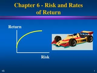
CHAPTER 6 Risk and Rates of Return • Stand-alone risk • Portfolio risk • Risk & return: CAPM/SML
Risk & Uncertainty Risk is seen as the phenomenon that arises from circumstances where we are able to identify the possible outcomes and even their likelihood of occurrence without being sure which will actually occur
Risk & Uncertainty The outcome of throwing a true die is an example of risk. We know that the outcome must be a number from 1 to 6 (inclusive) and we know that each number has an equal (1 in 6) chance of occurrence, but we are not sure which one will actually occur on any particular throw.
Risk & Uncertainty Uncertainty describes the position where we simply are not able to identify all, or perhaps not even any, of the possible outcomes, and we are still less able to assess their likelihood of occurrence. Probably most business decisions are characterized by uncertainty to some extent.
Risk & Uncertainty Uncertainty describes the position where we simply are not able to identify all, or perhaps not even any, of the possible outcomes, and we are still less able to assess their likelihood of occurrence. Probably most business decisions are characterized by uncertainty to some extent.
Risk & Uncertainty Uncertainty represents a particularly difficult area. Perhaps the best that decision makers can do is to try to identify as many as possible of the feasible outcomes of their decision and attempt to assess each outcome’s likelihood of occurrence.
Concept of Return The concept of return provides investors with a convenient way of expressing the financial performance of an investment.
Example of Return suppose you buy 10 shares of a stock for $1,000. The stock pays no dividends, but at the end of one year, you sell the stock for $1,100. What is the return on your $1,000 investment?
Expressing an Investment Return One way of expressing an investment return is in dollar terms. The dollar return is simply the total dollars received from the investment less the amount invested: Dollar return Amount received Amount invested =$1,100- $1,000 $100.
Limitations of Dollar returns Although expressing returns in dollars is easy, two problems arise: (1) To make a meaningful judgment about the return, you need to know the scale (size) of the investment; a $100 return on a $100 investment is a good return (assumingthe investment is held for one year), but a $100 return on a $10,000 investment would be a poor return
Limitations of Dollar returns (2) You also need to know the timing of the return; a $100 return on a $100 investment is a very good return if it occurs after one year, but the same dollar return after 20 years would not be very good.
Solution The solution to the scale and timing problems is to express investment results as rates of return, or percentage returns. For example, the rate of return on the 1-year stock investment, when $1,100 is received after one year, is 10 percent:
Explanation of Solution The rate of return calculation “standardizes” the return by considering the return per unit of investment. In this example, the return of 0.10, or 10 percent, indicates that each dollar invested will earn 0.10($1.00) $0.10.
Explanation of Solution The rate of return calculation “standardizes” the return by considering the return per unit of investment. In this example, the return of 0.10, or 10 percent, indicates that each dollar invested will earn 0.10($1.00) $0.10.
Explanation of Solution If the return had been negative, this would indicate that the original investment was not even recovered. For example, selling the stock for only $900 results in a 10 percent rate of return, which means that each dollar invested lost 10 cents.
Explanation of Solution Note also that a $10 return on a $100 investment produces a 10 percent rate of return, while a $10 return on a $1,000 investment results in a rate of return of only 1 percent. Thus, the percentage return takes account of the size of the investment
What is investment risk? Investment risk pertains to the probability of actually earning a low or negative return. The greater the chance of low or negative returns, the riskier the investment.
Type of risk? Stand-alone risk is the risk an investor would face if he or she held only this one asset. Obviously, most assets are held in portfolios, but it is necessary to understand stand-alone risk in order to understand risk in a portfolio context.
PROBABILITY DISTRIBUTIONS An event’s probability is defined as the chance that the event will occur. For example, a weather forecaster might state, “There is a 40 percent chance of rain today and a 60 percent chance that it will not rain.” If all possible events, or outcomes, are listed, and if a probability is assigned to each event, the listing is called a probability distribution. For our weather forecast, we could set up the ollowing probability distribution:
PROBABILITY DISTRIBUTIONS The possible outcomes are listed in Column 1, while the probabilities of these outcomes, expressed both as decimals and as percentages, are given in Column 2. Notice that the probabilities must sum to 1.0, or 100 percent. Probabilities can also be assigned to the possible outcomes (or returns) from an investment.
PROBABILITY DISTRIBUTIONS The possible outcomes are listed in Column 1, while the probabilities of these outcomes, expressed both as decimals and as percentages, are given in Column 2. Notice that the probabilities must sum to 1.0, or 100 percent. Probabilities can also be assigned to the possible outcomes (or returns) from an investment.
EXPECTED RATE OF RETURN If we multiply each possible outcome by its probability of occurrence and then sum these products, as in Table 6-2, we have a weighted average of outcomes. The weights are the probabilities, and the weighted average is the expected rate of return, kˆ , called “k-hat.” The expected rates of return for both Martin Products and U.S. Water are shown in Table 6-2 to be 15 percent. This type of table is known as a payoff matrix.
EXPECTED RATE OF RETURN The expected rate of return calculation can also be expressed as an equation that does the same thing as the payoff matrix table.
Calculate the expected rate of return on each alternative: ^ k = expected rate of return. ^
What’s the standard deviationof returns for each alternative? = Standard deviation. = = =
Standard deviation (si) measures total, or stand-alone, risk. • The larger the si , the lower the probability that actual returns will be close to the expected return. • The symbol for which is pronounced“sigma.” • The smaller the standard deviation, the tighter the probability distribution, and, accordingly, the lower the riskiness of the stock.
Standard Deviation Thus, the standard deviation is essentially a weighted average of the deviations from the expected value, and it provides an idea of how far above or below the expected value the actual value is likely to be.
Standard Deviation Martin’s standard deviation is seen in Table 6-3 to be 65.84%. Using these same procedures, we find U.S. Water’s standard deviation to be 3.87 percent. Martin Products has the larger standard deviation, which indicates a greater variation of returns and thus a greater chance that the expected return will not be realized.Therefore,Martin Products is a riskier investment than U.S. Water when held alone.
If a probability distribution is normal, the actual return will be within 1 standard deviation of the expected return 68.26 percent of the time. Figure 6-3 illustrates this point, and it also shows the situation for 2 and 3. For Martin Products, kˆ 15% and 65.84%, whereas kˆ 15% and 3.87% for U.S. Water. Thus, if the two distributions were normal, there would be a 68.26 percent probability that Martin’s actual return would be in the range of 15 +/- 65.84 percent, or from 50.84 to 80.84 percent. For U.S. Water, the 68.26 percent range is 15 +/- 3.87 percent, or from 11.13 to 18.87 percent. With such a small , there is only a small probability that U.S. Water’s return would be significantly less than expected, so the stock is not very risky
Coefficient of Variation (CV) Standardized measure of dispersion about the expected value: Std dev s CV = = . ^ Mean k Shows risk per unit of return.
Coefficient of Variation (CV) Standardized measure of dispersion about the expected value: Std dev s CV = = . ^ Mean k Shows risk per unit of return.
Prob. B A Rate of Return (%) 0 sA = sB , but A is riskier because larger probability of losses. s = CVA > CVB. ^ k
Portfolio Risk and Return Assume a two-stock portfolio with $50,000 in HT and $50,000 in Collections. ^ Calculate kp and sp.
Portfolio Return, kp ^ ^ kp is a weighted average: n ^ ^ kp = Swiki. i=1 ^ kp = 0.5(17.4%) + 0.5(1.7%) = 9.6%. ^ ^ ^ kp is between kHT and kCOLL.
Alternative Method Estimated Return Economy Prob. HT Coll. Port. Recession 0.10 -22.0% 28.0% 3.0% Below avg. 0.20 -2.0 14.7 6.4 Average 0.40 20.0 0.0 10.0 Above avg. 0.20 35.0 -10.0 12.5 Boom 0.10 50.0 -20.0 15.0 ^ kp = (3.0%)0.10 + (6.4%)0.20 + (10.0%)0.40 + (12.5%)0.20 + (15.0%)0.10 = 9.6%.
1 / 2 é ù ê ú (3.0 – 9.6)20.10 + (6.4 – 9.6)20.20 + (10.0 – 9.6)20.40 + (12.5 – 9.6)20.20 + (15.0 – 9.6)20.10 ê ú ê ú ê ú p= = 3.3%. ê ú ê ú ê ú ê ú ê ú ë û 3.3% CVp = = 0.34. 9.6%
sp = 3.3% is much lower than that of either stock (20% and 13.4%). • sp = 3.3% is lower than average of HT and Coll = 16.7%. • \ Portfolio provides average k but lower risk. • Reason: negative correlation. ^
General statements about risk • Most stocks are positively correlated. rk,m» 0.65. • s » 35% for an average stock. • Combining stocks generally lowers risk.
Returns Distributions for Two Perfectly Negatively Correlated Stocks (r = -1.0) and for Portfolio WM Stock W Stock M Portfolio WM . . . . 25 25 25 . . . . . . . 15 15 15 0 0 0 . . . . -10 -10 -10
25 25 15 15 0 0 -10 -10 Returns Distributions for Two Perfectly Positively Correlated Stocks (r = +1.0) and for Portfolio MM’ Stock M’ Portfolio MM’ Stock M 25 15 0 -10
What would happen to theriskiness of an average 1-stockportfolio as more randomlyselected stocks were added? • sp would decrease because the added stocks would not be perfectly correlated but kp would remain relatively constant. ^